Biomechanics and Medicine in Swimming XI

¾
¾
¾
Methods
A three-dimensional model of the fin-water system is proposed which
is built on the following assumptions. Based on continuum theory, a
fluid-structure interaction is developed with inertial coupling. The system
is depicted in Figure 1 and is composed of a solid domain (ΩS )
coupled with a surrounding fluid domain (ΩF ). The boundary (Γ) ¾
corresponds to the deformable fluid-structure interface. The external
excitation for the stroke motion (i.e. the rate of undulation) ¾ is assumed
to be lower than the wave speed ¾ in the fin, so that the fluid can be ¾ de-
¾
scribed with the acoustic pressure (Morand and Ohayon, 1995). It corresponds
to an undulatory type of low frequency swimming. The fin is
assumed to be a deformable elastic structure. Namely, the monofin is
modelled using a multilayer structure, whose constitutive law is written
by means of the Cauchy stress tensorσ
. The imposed kinematics at the
leading edge of the monofin (that corresponds to the swimmer’s ankle)
results in a volume force γ ie. If we denote by u the displacement field of
the monofin and p pressure field within the fluid domain, the problem
consists in finding (u,p) solutions of the following three-dimensional
¾
boundary value problem:
¾
r ∂ 2 u
∂t 2 u
=
=
divσ + γ ie
0
(ΩS )
(Γ0 )
(1)
(2)
σ.n = −pn (Γ) (3)
∆p − 1
2
c0 ∂ 2 p
∂t 2 = div(−r 0γ ie) (Ω F ) (4)
∂p
∂
= −r0 ∂n
2 u
∂t 2 .n − r0γ ie.n (Γ1) (5)
∂p
= −r0γ ie.n (Γ) (6)
∂n
¾
p = 0 (Γg ∪ Γs ∪ Γe) (7)
xω(t) + zω
γ ie =
2 (t)
0
zω(t) − xω 2 ⎡
⎤
⎢
⎥
⎢
⎥
⎣
⎢ (t) ⎦
⎥
Where c is the wave velocity in the fluid, r is the density of the mono-
0 ¾
fin, r is the fluid density and n is the unit outward normal to the fin
0
domain. The coupling results in a new term in the inertial contribution of
the system. Indeed, this added mass characterizes the energy transmission
¾
between the fin and the water. The specificity of the present method is that
¾
the temporal evolution ¾ of dynamical features is available. Namely, transient
added mass, three-dimensional forces and torques at the point corresponding
to the swimmer’s ankle as well as energy balance are obtained.
Since this resulting fluid-structure interaction problem is too complex to
be solved analytically, we analyzed using the means of numerical approximation.
We will briefly outline the solution methodology used to solve
the governing equations. The latter are solved with the Finite Element
Method using the commercial software COMSOL Multiphysics (Comsol
Inc., Burlington, USA) . Numerical simulations are carried out for the
fluid flow in a pool with the following dimensions: In the pool, a fin with
realistic dimensions (0.80 m chord and 0.50 wide) is located at the distance
of 5 m from left wall. In this study a monolithic approach is used.
Indeed, the equations governing the fluid flow and the displacement of the
structure are solved simultaneously with single solver. The main steps of
the methodology are the following: first, based on realistic pictures, the
geometry of the monofin is created. The resulting volume, which is the
form of an Initial Graphics Exchange Specification (IGES) file format,
is then input into the commercial software COMSOL Multiphysics and
transformed to an unstructured volume mesh with triangular elements.
The second step consists in the meshing. The final volume mesh (Figure
1) consists of 6256 triangular elements for the fin and 128676 triangular
elements for the water. The third step consists in a modal analysis of the
three-dimensional coupled problem. γ ie is set to zero and a time harmonic
solution of the problem is computed. This allows obtaining the fundamental
vibration characteristics of the immersed monofin and therefore
the quantitative and qualitative effect of the added mass can be pointed
out. The final step of the ¾ methodology consists in a transient analysis of
propulsive forces. Thus, in the numerical experiments that are presented,
the monofin is undergoing time-dependent motion that combines translating
and rotating motions as follows
chaPter2.Biomechanics
ω(t) = θ0 sin(ω 0t +ψ) h(t) = h0 sin(ω 0t)
with
ω0 =1.7rad.s −1
θ0 = π
rad
4
π
ψ =
2 rad h0 = 3
4 c
in which c is the chord of the monofin. In the numerical experiments, c
is set to 0.7m. The material properties used in the FEM simulation are
given in Table 1.
Table 1. Material characteristics used in the FEM simulation. E is the
Young’s modulus, ν is the Poisson’s coefficient and r is the density of
the monofin. (Data provided by Breier SAS company)
¾
E [Pa] ν
r [kg.m
¾
¾
¾ ¾
¾ ¾
¾
−3 ]
Carbon 12K
146.10
¾
9
0.32 1565
Low density Polyethylene 146.10
¾ ¾
¾
9
0.38 920
Rubber
0,05.10
¾ ¾
¾
9 0.49 1250
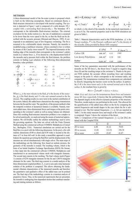
Some of the key parameters associated with the performance of the
monofin are the lift force L, the thrust ¾ force ¾ T (equal to negative drag
force D) and the resulting torque at the swimmer’s. Thanks to the present
FEM method, the accurate efforts (resulting force and resulting
torque) at the point O, which corresponds to the swimmer ankle, are
computed. The instantaneous resultant force components are calculated
by directly integrating the traction vector on the fin surface. In particular,
if σ is the stress tensor and n is the outward normal unit to the fin
surface A, the resultant force is given by
R(t) = ∫ σ.ndΓ
= L(t).x + L(t).z
A
where T(t) and L(t) are the instantaneous thrust force and instantaneous
lift force respectively. It known that the performance of flexible
fins depends largely on the effective dynamic properties of the structure.
Therefore, ¾ modal analysis was performed in this work. This allowed for
¾
the quantification of the added mass effect on the fin by comparing the
natural frequencies and modal shapes in the case where the fin is submerged
or not. The first natural frequencies fi = λi /2π are reported in
Table 2. In this study transient force and torque at the swimmer’s ankle
is computed. Figure 3 shows the variation of the thrust.
Table 2. Comparison of first natural frequencies fi = λi /2π [Hz] obtained
with the Coupled FEM. ¾
f1 f2 f3
2D in water 6.08 41.12 70.03
3D in vacuum 13.01 ¾ 113.51 256.34
3D in water 4.395 23.87 41.87
53