- Page 1 and 2:
Energy Systems and Technologies for
- Page 3 and 4:
ContentsSessions overview 1Programm
- Page 5 and 6:
sessions overview08:00-09:00Coffee
- Page 7 and 8:
11:00 - 12:30 session 6A - Bioenerg
- Page 9 and 10:
ContactSustainable Energy, Technica
- Page 11 and 12:
Penetration of new energy technolog
- Page 13 and 14:
how decisions are made and by whom
- Page 15 and 16:
(9) is the logaritimic expansion of
- Page 17 and 18:
(16)we may finally write Eq(14) in
- Page 19 and 20:
Table 1: Fast track cases for new r
- Page 21 and 22:
Peterka V. Macrodynamics of technol
- Page 23 and 24:
Growth in clean and reliable energy
- Page 25 and 26:
Conclusion - an ambitious vision an
- Page 27 and 28:
"Spurring investments in renewable
- Page 29 and 30:
Integrating climate change adaptati
- Page 31 and 32:
transport, and finance. Energy prov
- Page 33 and 34:
northern South America, the Caribbe
- Page 35 and 36:
Table 1: Energy system adaptation s
- Page 37 and 38:
More generally, a number of no- or
- Page 39 and 40:
6 ReferencesADB, 2005. Climate proo
- Page 41 and 42:
Sailor, D.J., Smith, M., Hart, M.,
- Page 43 and 44:
Factors affecting stakeholder perce
- Page 45 and 46:
Another study conducted in Japan wa
- Page 47 and 48:
4 The effect of information on stak
- Page 49 and 50:
Furthermore, communication to stake
- Page 51 and 52:
Shackley S, McLachlan C, Gough C (2
- Page 53 and 54:
Figure 1: Potential CO 2 storage si
- Page 55 and 56:
The Upper Jurassic - Lower Cretaceo
- Page 57 and 58:
The majority of the individual stru
- Page 59 and 60:
Development. Project no. ENK6-CT-19
- Page 61 and 62:
Section 5 summarises the key issue
- Page 63 and 64:
Table 1. Efficiencies for new large
- Page 65 and 66:
In addition, district heating syste
- Page 67 and 68:
6.4 Model results from EFDA-TIMESIn
- Page 69 and 70:
Maisonnier, D., et al. (2007), Powe
- Page 71 and 72:
1Efficiency and effectiveness of pr
- Page 73 and 74:
3Stromerzeugung [TWh/a]250200150100
- Page 75 and 76:
54 Country-specific Lessons learned
- Page 77 and 78:
7100%90%80%quota fullfilment (%)70%
- Page 79 and 80:
[5] Haas R., et al: Efficiency and
- Page 81 and 82:
The development and diffusion of re
- Page 83 and 84:
a. Offshore wind in DenmarkDenmark
- Page 85 and 86:
applicants are invited to submit a
- Page 87 and 88:
nies that provide upstream and down
- Page 89 and 90:
for both technology users and produ
- Page 91 and 92:
Trade Disputes over Renewable Energ
- Page 93 and 94:
treatment to imported renewable ene
- Page 95 and 96:
In Canada, the federal government i
- Page 97 and 98:
grid access, subsidies and land off
- Page 99 and 100:
In 2010, China’s total wind insta
- Page 101 and 102:
Source: Renewables 2010 Global Stat
- Page 103 and 104:
Source: REN 21, Renewables 2010 Glo
- Page 105 and 106:
Source: adapted from REN21, 2010It
- Page 107 and 108:
their precise scope and nature diff
- Page 109 and 110:
60 daysBy 2 nd DSBmeetingConsultati
- Page 111 and 112:
discriminatory manner on domestic a
- Page 113 and 114:
the European Union, the North Ameri
- Page 115:
ended. China lost this case because
- Page 118 and 119:
As most countries in the world are
- Page 120 and 121:
Session 3A - Energy SystemsRisø In
- Page 122 and 123:
1 IntroductionWith the introduction
- Page 124 and 125: occur. This is an undesirably burea
- Page 126 and 127: This curve could be used as a new t
- Page 128 and 129: ut for the total consumption, and i
- Page 130 and 131: This gives the LBR an opportunity t
- Page 132 and 133: concludes that the subsurface conta
- Page 134 and 135: to constrain the evaluation. In add
- Page 136 and 137: Fig. 2 SW-NE trending seismic profi
- Page 138 and 139: Fig. 5. Petrophysical evaluation of
- Page 140 and 141: ConclusionsThe Danish subsurface co
- Page 142 and 143: Performance of Space Heating in aMo
- Page 144 and 145: [5],[10],[11],[16],[18],[20],[26].
- Page 146 and 147: 2/3 Sun1 Coal1/3 ElPower plantHP1 H
- Page 148 and 149: 25002000Surplus(min(wind,prod-cons)
- Page 150 and 151: 160CO 2 emission per unit heat prod
- Page 152 and 153: The calculations have been based on
- Page 154 and 155: Session 3B - smart gridsRisø Inter
- Page 156 and 157: 2 Myopic Investments2.1 The Balmore
- Page 158 and 159: Moreover, this model is formulated
- Page 160 and 161: Reducing Electricity Demand Peaks b
- Page 162 and 163: 3 Event Driven Scheduling Algorithm
- Page 164 and 165: 5 Mapping Teletraffic Theory to Ene
- Page 166 and 167: 6.2 Results and Performance Metrics
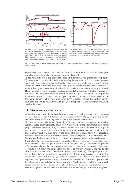
- Page 168 and 169: Energy Efficient Refrigeration and
- Page 170 and 171: Virtual Power PlantAggregatorSuperm
- Page 172 and 173: C p,rC p,fT rT fW cφ sT a(UA) raHe
- Page 176 and 177: the availability payment.Simulation
- Page 178 and 179: The constraint in Eq. (16) has the
- Page 180 and 181: The FlexControl concept - a vision,
- Page 182 and 183: can react on requests for power reg
- Page 184 and 185: 3 ControlThe concept is based solel
- Page 186 and 187: one hour to the next - correspondin
- Page 188 and 189: 4 ProtectionThe protection of the p
- Page 190 and 191: Session 4 - Efficiency Improvements
- Page 192 and 193: the product portfolio point of view
- Page 194 and 195: Figure 4: Principle flow sheet of t
- Page 196 and 197: process information needed are seld
- Page 198 and 199: AIRFINE®(Reference)MEROS®Ca(OH)2M
- Page 200 and 201: 4 Conclusion & DiscussionThe Eco-Ca
- Page 202 and 203: 1 Energy policy and EU directivesTh
- Page 204 and 205: iomass CHP, heat pumps, electric bo
- Page 206 and 207: Fig. 1: How to supply a growing hea
- Page 208 and 209: Session 5A - Wind Energy IRisø Int
- Page 210 and 211: The average cumulative growth rate
- Page 212 and 213: turbines is expected to create a st
- Page 214 and 215: O&MGridWindturbineSubstructureFigur
- Page 216 and 217: Another idea is to harvest energy f
- Page 218 and 219: 9. Shimon Awerbuch, Determining the
- Page 220 and 221: engaged in wind energy assessment,
- Page 222 and 223: treated in such a way to make them
- Page 224 and 225:
Figure 5: Map showing the estimated
- Page 226 and 227:
Figure 9: The annual mean power den
- Page 228 and 229:
mix is required. For example diurna
- Page 230 and 231:
Session 5B - Wind Energy IIRisø In
- Page 232 and 233:
TABLE ISOME OF THE WIND TURBINE MAN
- Page 234 and 235:
China, has prompted all parties, in
- Page 236 and 237:
to the high shaft speed. Furthermor
- Page 238 and 239:
Superconductors must be kept cold b
- Page 240 and 241:
an annual increase in demand of 6%,
- Page 242 and 243:
Improved High Temperature Supercond
- Page 244 and 245:
our study to a single set of deposi
- Page 246 and 247:
3.2 Yttrium-enriched YBCO thin film
- Page 248 and 249:
Fig. 5. AC-susceptibility dependenc
- Page 250 and 251:
The j C (B) dependence at 50 K for
- Page 252 and 253:
Session 6A - Bioenergy IRisø Inter
- Page 254 and 255:
The European politicians are faced
- Page 256 and 257:
The fast growing demand for biomass
- Page 258 and 259:
Figure 2: Avedøre Power Plant in C
- Page 260 and 261:
Figure 5: Concept for a sustainable
- Page 262 and 263:
The role of biomass and CCS in Chin
- Page 264 and 265:
2.2.1 CCS Potential for ChinaCCS is
- Page 266 and 267:
80%70%60%China's share ofglobal CO
- Page 268 and 269:
In general, if the CCS technology d
- Page 270 and 271:
with high implementation of CCS Chi
- Page 272 and 273:
The European Biofuels Policy: from
- Page 274 and 275:
aimed to promote agriculture-based
- Page 276 and 277:
(EC, 2009b), and internationally vi
- Page 278 and 279:
Session 6B - Bio Energy IIRisø Int
- Page 280 and 281:
The commercial scale production of
- Page 282 and 283:
the production process parameters,
- Page 284 and 285:
NutrientWaterAlgal cultureproductio
- Page 286 and 287:
Schenk, P.M., Thomas-Hall, S.R., St
- Page 288 and 289:
Liquid biofuels from blue biomassZs
- Page 290 and 291:
Even though final ethanol yields we
- Page 292 and 293:
Integrated Gasification SOFC Plant
- Page 294 and 295:
2.1 Modelling of SOFCThe SOFC model
- Page 296 and 297:
where g 0 , R an T are the specific
- Page 298 and 299:
hand side y-axis corresponds to eff
- Page 300 and 301:
The moister content for these three
- Page 302 and 303:
Use of Methanation for Optimization
- Page 304 and 305:
power production from utilizing the
- Page 306 and 307:
2.1 Model DescriptionThe developed
- Page 308 and 309:
Figure 3: Flow sheet of methanation
- Page 310 and 311:
efficiency and turbine inlet temper
- Page 312 and 313:
[14] DNA - A Thermal Energy System
- Page 314 and 315:
On the effectiveness of standards v
- Page 316 and 317:
educing new car emissions to 120 g
- Page 318 and 319:
In addition energy consumption E an
- Page 320 and 321:
coefficient γ for the impact of fu
- Page 322 and 323:
400200Change in energy (PJ)01980 19
- Page 324 and 325:
Figure 9 depict scenarios for the f
- Page 326 and 327:
What are customers willing to pay f
- Page 328 and 329:
Randomly, continuous up to ±50%Acc
- Page 330 and 331:
The likelihood for the model is giv
- Page 332 and 333:
eally means that this factor and no
- Page 334 and 335:
Table 5-1 Parameter estimates from
- Page 336 and 337:
Table 6-2 Willingness to pay for 10
- Page 338 and 339:
Session 12 - Energy for Developing
- Page 340 and 341:
Risø International Energy Conferen
- Page 342 and 343:
Risø International Energy Conferen
- Page 344 and 345:
Risø International Energy Conferen
- Page 346 and 347:
Risø International Energy Conferen
- Page 348 and 349:
Risø International Energy Conferen
- Page 350 and 351:
existing renewable energy technolog
- Page 352 and 353:
useful energyend energysecondary en
- Page 354 and 355:
parts or the means of enforcing war
- Page 356 and 357:
The development of micro-hydro proj
- Page 358 and 359:
Table 1. Electric power generation
- Page 360 and 361:
5 ReferencesBajgain, S., Shakya, I.
- Page 362 and 363:
IntroductionElectricity has become
- Page 364 and 365:
of 2008, 43.6% of the total populat
- Page 366 and 367:
Hilmand provinces have comparativel
- Page 368 and 369:
….. eq. 5LCOE is the net present
- Page 370 and 371:
case of Nepal, it is 5% (Trading ec
- Page 372 and 373:
ing down the cost of solar PV modul
- Page 374 and 375:
3.3 Serving the rural areas with na
- Page 376 and 377:
The levelized costs of electricity
- Page 378 and 379:
Figure 4. Variation in LCOE with si
- Page 380 and 381:
The analysis reveals that fuel cost
- Page 382 and 383:
In case of DG, we have looked with
- Page 384 and 385:
Gross, R., Blyth, W., Heptonstall,
- Page 386 and 387:
Mode of Transport to Work, Car Owne
- Page 388 and 389:
power parity (PPP) basis, GDP per c
- Page 390 and 391:
83,385 to 109,108 while the number
- Page 392 and 393:
other purposes so that reduced fare
- Page 394 and 395:
emissions studies is that they were
- Page 396 and 397:
where I (·) is the indicator funct
- Page 398 and 399:
increases, individuals acquire more
- Page 400 and 401:
while that of other means of transp
- Page 402 and 403:
into CO 2 . For all oil and oil pro
- Page 404 and 405:
impact. In general, income is found
- Page 406 and 407:
7 ReferenceAlperovich, G., Deutsch,
- Page 408 and 409:
Table 1: Definitions of Variables a
- Page 410 and 411:
Session 13 - Energy StorageRisø In
- Page 412 and 413:
2 Storage demand and resulting stor
- Page 414 and 415:
compressed air storages, demand sit
- Page 416 and 417:
Fig. 3: Options for underground sto
- Page 418 and 419:
3.5 Geological potential in EuropeF
- Page 420 and 421:
Sensitivity on Battery Prices and C
- Page 422 and 423:
3.1 Base caseA northern European en
- Page 424 and 425:
4 ResultsThe model is run on a comp
- Page 426 and 427:
Furthermore, a slight decrease in t
- Page 428 and 429:
Night time charging increases with
- Page 430 and 431:
Lithuanian Energy Institute, PSE In
- Page 432 and 433:
atteries, Compressed Air Energy Sto
- Page 434 and 435:
negative net load, can be expected
- Page 436 and 437:
25%Pct. of the year20%15%10%5%0.5-0
- Page 438 and 439:
800006000040000MWh200000Netload-200
- Page 440 and 441:
[4] B. V. Mathiesen and H. Lund, "C
- Page 442 and 443:
Compressed Air Energy Storage in Of
- Page 444 and 445:
compressed air caverns, corrosion-r
- Page 446 and 447:
Figure 3: Distribution of salt depo
- Page 448 and 449:
Figure 6: EWEA's 20 year Offshore N
- Page 450 and 451:
spinning reserves can be provided b
- Page 452 and 453:
7 Discussion and conclusionsThis pa
- Page 454:
Risø DTU is the National Laborator