Immersioni aperte in dimensione infinita - Dipartimento di Matematica

D.6 Costruzione di una filtrazione totalmente geodetica 95
Analogamente alla nozione di pull-back di una metrica (cfr. definizione 1.4) si introduce la
seguente comoda
Definizione D.22. Sia (M, g) una varietà Riemanniana ed f : M → N un diffeomorfismo tra M
ed una varietà N. Il push-forward della metrica g mediante f è la metrica df(g) su N definita
ponendo
−1 −1
df(g)p(X, Y ) := gf −1 (p) df (X), df (Y ) .
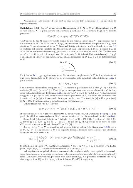
Costruzione 1. Sia M una sottovarietà chiusa di una varietà Hilbertiana N. Supponiamo che il
fibrato normale di M in N sia banale. Sia g M una struttura Riemanniana completa su M e g N una
struttura Riemanniana completa su N. Sono soddisfatte le ipotesi di applicabilità del teorema D.8
di esistenza dell’intorno tubolare. Inoltre, siccome abbiamo supposto che il fibrato normale di M in
N sia banale, sfruttando la metrica g N possiamo costruire un intorno tubolare di M in N della forma
ϕ: M × H → U, in cui U è un aperto di N contenente M (il tubo dell’intorno tubolare), (H, g H )
è uno spazio di Hilbert di dimensione eguale alla codimensione di M in N e ϕ è un diffeomorfismo
su U
M × H
ϕ
π M
M
ι
U
(D.6.2)
Per il lemma D.21, g M ×g H è una struttura Riemanniana completa su M ×H; inoltre tale struttura
può essere trasportata su U attraverso ϕ, precisamente, nelle notazioni della definizione D.22, il
push-forward
g U := dϕ(g M × g H) (D.6.3)
è una metrica Riemanniana completa su U. Si osservi in particolare che le fibre ϕ({x} × H) e le
sezioni ϕ(M ×{ξ}) (∀x ∈ M, ξ ∈ H) di (U, gU ) sono rispettivamente isometriche ad H e M; inoltre,
come nella dimostrazione del lemma D.21, ogni curva C 1 a tratti da (x, ξ1) a (x, ξ2) ha lunghezza
maggiore o al più uguale della corrispondente curva proiettata su H. Ne deriva che la distanza fra
i punti (x, ξ1) e (x, ξ2) può essere calcolata a partire da curve C 1 a tratti in {x} × H oppure (aut)
in M × {ξ}. Denotiamo con ρ H la metrica su H associata a g H .
Consideriamo per δ in R + l’insieme
Uδ := ϕ(M × δH) = ϕ(x, ξ) : (x, ξ) ∈ M × H ∧ |ξ | < δ . (D.6.4)
(La notazione M × δH è già stata introdotta all’interno della tesi, cfr. Notazione 2.54 pag. 41.) In
particolare Uδ è un intorno tubolare di M, ma non è un intorno tubolare totale (cfr. definizione D.6).
Siano f1 ed f2 funzioni definite su H tali che f1 ≡ 1 su {ξ : |ξ | ≤ 4}, f1 ≡ 0 su {ξ : |ξ | ≥ 5};
f2 ≡ 0 su {ξ : |ξ | ≤ 2}, f2 ≡ 1 su {ξ : |ξ | ≥ 3}. Si noti che f1 ed f2 possono essere scelte di classe
C ∞ perché la norma su H è di classe C ∞ su H \ {0}.
Sia π H : M × H → H la proiezione sul secondo fattore, allora (cfr. diagramma D.6.2) per y
in U, π H (ϕ −1 (y)) appartiene a H e la seguente formula definisce correttamente una struttura
Riemanniana sulla varietà N:
h(y) : def
=
−1 −1
f1 πH ϕ (y) gU (y) + f2 πH ϕ (y) gN (y) se y ∈ U,
gN (y) se y ∈ N \ U.
(D.6.5)
Si noti che h è di classe C ∞ , infatti per costruzione h ≡ g N su N \ U5 e gN è di classe C ∞ ; d’altra
parte, se y ∈ U6 ⊂ U, la formula che definisce h(y) è di classe C ∞ .
Nel seguito saremo principalmente interessati alla lunghezza delle curve, quindi sarà comodo
usare la notazione h, g U , g N , g M per indicare la forma quadratica associata alle corrispondenti metriche.
Con questa convenzione, per come sono state definite g U e h, possiamo affermare che su U4
risulta g U ≤ h, su U c 3 := N \ U3, g N ≤ h ed infine su U4 ∩ U c 3, h = g U + g N .
RAUL TOZZI