Immersioni aperte in dimensione infinita - Dipartimento di Matematica

44 Embedding aperti di varietà di dimensione infinita
Il prossimo obiettivo sarà la costruzione di una funzione globale “r” definita su tutta la varietà
M, r ∈ C(M, R + ), in modo tale che, per ogni n in N, Dn = Mn × r|MnH n sia un intorno standard
di Mn. Questa costruzione sarà affrontata nella dimostrazione della proposizione 2.63: sfrutteremo
alcune delle idee che abbiamo utilizzato per dimostrare la proposizione precedente, inoltre, come è
facile intuire, le partizioni dell’unità saranno il mezzo tecnico per definire una funzione continua r
globalmente definita sulla varietà.
Prima di affrontare questa costruzione che, seppure tecnica, è veramente molto interessante –si
percepisce come tutti gli ingredienti che abbiamo introdotto fino a questo punto si combinino l’uno
con l’altro in modo ineccepibile e conclusivo– cercheremo di rispondere alla seguente domanda:
fissato x0 in M, quanto può essere grande r(x0) ? Chiaramente la sua grandezza dipende in primo
luogo dal raggio della palletta centrata in x0 su cui la mappa Tn è localmente invertibile. Vedremo
come si ottiene la palletta dal teorema di inversione locale e forniremo una stima uniforme in n
sul raggio. Precisamente, indicato con x0 in M un punto generico, determineremo un intorno Ax 0
uniforme in n su cui Tn risulterà iniettiva, cosa che non stupisce dato che le Tn sono tutte molto
simili fra loro. Dunque studieremo anche quanto ridurre r(x0) in modo da ottenere un aperto su
cui Tn è iniettiva.
Una risposta esaustiva a tutto questo è contenuta nella dimostrazione del seguente lemma:
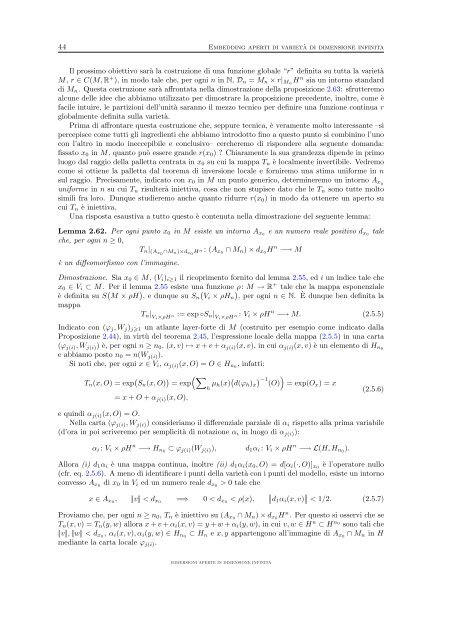
Lemma 2.62. Per ogni punto x0 in M esiste un intorno Ax0 e un numero reale positivo dx0 tale
che, per ogni n ≥ 0,
Tn| (Ax0 ∩Mn)×dx 0 H n : (Ax0 ∩ Mn) × dx0 Hn −→ M
è un diffeomorfismo con l’immagine.
Dimostrazione. Sia x0 ∈ M, (Vi)i≥1 il ricoprimento fornito dal lemma 2.55, ed i un indice tale che
x0 ∈ Vi ⊂ M. Per il lemma 2.55 esiste una funzione ρ: M → R + tale che la mappa esponenziale
è definita su S M × ρH
, e dunque su Sn Vi × ρHn , per ogni n ∈ N. È dunque ben definita la
mappa
Tn| Vi×ρH n := exp ◦Sn| Vi×ρH n : Vi × ρH n −→ M. (2.5.5)
Indicato con (ϕj, Wj)j1 un atlante layer-forte di M (costruito per esempio come indicato dalla
Proposizione 2.44), in virtù del teorema 2.45, l’espressione locale della mappa (2.5.5) in una carta
(ϕj(i), Wj(i)) è, per ogni n ≥ n0, (x, v) ↦→ x + v + αj(i)(x, v), in cui αj(i)(x, v) è un elemento di Hn0
e abbiamo posto n0 = n(Wj(i)). Si noti che, per ogni x ∈ Vi, αj(i)(x, O) = O ∈ Hn0 , infatti:
Tn(x, O) = exp Sn(x, O)
= exp
h µh(x)
−1(O)
d(ϕh)x = exp(Ox) = x
= x + O + αj(i)(x, O),
(2.5.6)
e quindi α j(i)(x, O) = O.
Nella carta (ϕ j(i), W j(i)) consideriamo il differenziale parziale di αi rispetto alla prima variabile
(d’ora in poi scriveremo per semplicità di notazione αi in luogo di α j(i)):
αi : Vi × ρH n −→ Hn0 ⊂ ϕ j(i)(W j(i)), d1αi : Vi × ρH n −→ L(H, Hn0).
Allora (i) d1αi è una mappa continua, inoltre (ii) d1αi(x0, O) = d[αi(·, O)]x0 è l’operatore nullo
(cfr. eq. 2.5.6). A meno di identificare i punti della varietà con i punti del modello, esiste un intorno
convesso Ax0 di x0 in Vi ed un numero reale dx0 > 0 tale che
x ∈ Ax0 , |v | < dx0 =⇒ 0 < dx0 < ρ(x),
d1αi(x, v) < 1/2. (2.5.7)
Proviamo che, per ogni n ≥ n0, Tn è iniettivo su (Ax0 ∩ Mn) × dx0 Hn . Per questo si osservi che se
Tn(x, v) = Tn(y, w) allora x + v + αi(x, v) = y + w + αi(y, w), in cui v, w ∈ H n ⊂ H n0 sono tali che
|v |, |w | < dx0, αi(x, v), αi(y, w) ∈ Hn0 ⊂ Hn e x, y appartengono all’immagine di Ax0 ∩ Mn in H
mediante la carta locale ϕ j(i).
IMMERSIONI APERTE IN DIMENSIONE INFINITA