TH`ESE DE DOCTORAT DE L'UNIVERSITà PARIS 6 Spécialité ...
TH`ESE DE DOCTORAT DE L'UNIVERSITà PARIS 6 Spécialité ...
TH`ESE DE DOCTORAT DE L'UNIVERSITà PARIS 6 Spécialité ...

You also want an ePaper? Increase the reach of your titles
YUMPU automatically turns print PDFs into web optimized ePapers that Google loves.
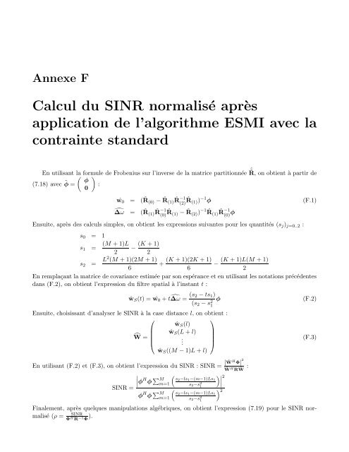
Annexe F<br />
Calcul du SINR normalisé après<br />
application de l’algorithme ESMI avec la<br />
contrainte standard<br />
En utilisant la ( formule ) de Frobenius sur l’inverse de la matrice partitionnée ˆ˜R, on obtient à partir de<br />
(7.18) avec ˜φ φ<br />
= :<br />
0<br />
ŵ 0 = ( ˆR (0) − ˆR ˆR−1 ˆR (1) (2) (1) ) −1 φ (F.1)<br />
̂∆ω = ( ˆR ˆR−1 ˆR (1) (0) (1) − ˆR (2) ) −1 ˆR(1) ˆR−1 (0) φ<br />
Ensuite, après des calculs simples, on obtient les expressions suivantes pour les quantités (s j ) j=0..2 :<br />
s 0 = 1<br />
(M + 1)L (K + 1)<br />
s 1 = −<br />
2 2<br />
s 2 = L2 (M + 1)(2M + 1) (K + 1)(2K + 1) (K + 1)L(M + 1)<br />
+ −<br />
6<br />
6<br />
2<br />
En remplaçant la matrice de covariance estimée par son espérance et en utilisant les notations précédentes<br />
dans (F.2), on obtient l’expression du filtre spatial à l’instant t :<br />
ŵ S (t) = ŵ 0 + t̂∆ω = (s 2 − ts 1 )<br />
(s 2 − s 2 φ<br />
1<br />
Ensuite, choisissant d’analyser le SINR à la case distance l, on obtient :<br />
⎛<br />
Ŵ = ⎜<br />
⎝<br />
ŵ S (l)<br />
ŵ S (L + l)<br />
.<br />
ŵ S ((M − 1)L + l)<br />
En utilisant (F.2) et (F.3), on obtient l’expression du SINR : SINR = |ŴH Φ| 2<br />
SINR =<br />
∣<br />
∣φ H φ ∑ M<br />
φ H φ ∑ M<br />
m=1<br />
⎞<br />
⎟<br />
⎠<br />
(<br />
s2 −ls 1 −(m−1)Ls 1<br />
m=1 s 2 −s 2 1<br />
( ) 2<br />
s2 −ls 1 −(m−1)Ls 1<br />
s 2 −s 2 1<br />
)∣ ∣∣<br />
2<br />
Ŵ H RŴ :<br />
Finalement, après quelques manipulations algébriques, on obtient l’expression (7.19) pour le SINR normalisé<br />
(ρ =<br />
SINR<br />
Φ H R −1 Φ ).<br />
(F.2)<br />
(F.3)