- Page 2 and 3:
Modern Engineering Thermodynamics
- Page 4 and 5:
Modern Engineering Thermodynamics R
- Page 6 and 7:
Dedication WHAT IS AN ENGINEER AND
- Page 8 and 9:
Contents PREFACE . . . . . . . . .
- Page 10 and 11:
Contents ix 7.6 Heat Engines Runnin
- Page 12 and 13:
Contents xi 14.13 Air Standard Gas
- Page 14 and 15:
Preface TEXT OBJECTIVES This textbo
- Page 16 and 17:
Preface xv Step 5. Write down the b
- Page 18 and 19:
Acknowledgments I wish to acknowled
- Page 20 and 21:
Resources That Accompany This Book
- Page 22 and 23:
List of Symbols A a B COP CR c c p
- Page 24 and 25:
Prologue PARIS FRANCE, 10:35 AM, AU
- Page 26 and 27:
CHAPTER 1 The Beginning CONTENTS 1.
- Page 28 and 29:
1.2 Why Is Thermodynamics Important
- Page 30 and 31:
1.3 Getting Answers: A Basic Proble
- Page 32 and 33:
1.5 How Do We Measure Things? 7 bei
- Page 34 and 35:
1.6 Temperature Units 9 THE DEVELOP
- Page 36 and 37:
1.7 Classical Mechanical and Electr
- Page 38 and 39:
1.7 Classical Mechanical and Electr
- Page 40 and 41:
1.9 Modern Units Systems 15 where M
- Page 42 and 43:
1.10 Significant Figures 17 CRITICA
- Page 44 and 45:
1.10 Significant Figures 19 WHAT AB
- Page 46 and 47:
1.11 Potential and Kinetic Energies
- Page 48 and 49:
1.11 Potential and Kinetic Energies
- Page 50 and 51:
Summary 25 FIGURE 1.19 Case study 1
- Page 52 and 53:
Problems 27 Problems (* indicates p
- Page 54 and 55:
Problems 29 14. Determine the mass
- Page 56 and 57:
Problems 31 49. Using the CGS units
- Page 58 and 59:
CHAPTER 2 Thermodynamic Concepts CO
- Page 60 and 61:
2.3 Phases of Matter 35 System boun
- Page 62 and 63:
2.4 System States and Thermodynamic
- Page 64 and 65:
2.6 Thermodynamic Processes 39 WHAT
- Page 66 and 67:
2.7 Pressure and Temperature Scales
- Page 68 and 69:
2.9 The Continuum Hypothesis 43 Sur
- Page 70 and 71:
2.10 The Balance Concept 45 Solutio
- Page 72 and 73:
2.11 The Conservation Concept 47 or
- Page 74 and 75:
2.11 The Conservation Concept 49 Th
- Page 76 and 77:
Summary 51 change in the mass of X
- Page 78 and 79:
Problems 53 Problems (* indicates p
- Page 80 and 81:
Problems 55 and Death rate = α 2 +
- Page 82 and 83:
CHAPTER 3 Thermodynamic Properties
- Page 84 and 85:
3.3 Fun with Mathematics 59 CRITICA
- Page 86 and 87:
3.4 Some Exciting New Thermodynamic
- Page 88 and 89:
3.6 Enthalpy 63 WHO WAS AMALIE EMMY
- Page 90 and 91:
3.7 Phase Diagrams 65 WHO WAS EMMY
- Page 92 and 93:
Pressure Vapor 3.7 Phase Diagrams 6
- Page 94 and 95:
3.7 Phase Diagrams 69 WHAT IS A “
- Page 96 and 97:
3.7 Phase Diagrams 71 considerable
- Page 98 and 99:
3.8 Quality 73 10 5 300 C Critical
- Page 100 and 101:
3.8 Quality 75 Although Eq. (3.26)
- Page 102 and 103:
3.9 Thermodynamic Equations of Stat
- Page 104 and 105:
3.9 Thermodynamic Equations of Stat
- Page 106 and 107:
3.9 Thermodynamic Equations of Stat
- Page 108 and 109:
3.9 Thermodynamic Equations of Stat
- Page 110 and 111:
3.10 Thermodynamic Tables 85 Critic
- Page 112 and 113:
3.12 Thermodynamic Charts 87 vð100
- Page 114 and 115:
3.13 Thermodynamic Property Softwar
- Page 116 and 117:
Summary 91 and e = E/m = u + V2 2g
- Page 118 and 119:
Problems 93 c. For a saturated mixt
- Page 120 and 121:
Problems 95 specific enthalpy of sa
- Page 122 and 123:
Problems 97 Table 3.23 Problem 65 M
- Page 124 and 125:
CHAPTER 4 The First Law of Thermody
- Page 126 and 127:
4.3 The First Law of Thermodynamics
- Page 128 and 129:
4.3 The First Law of Thermodynamics
- Page 130 and 131:
4.4 Energy Transport Mechanisms 105
- Page 132 and 133:
4.5 Point and Path Functions 107 4.
- Page 134 and 135:
4.6 Mechanical Work Modes of Energy
- Page 136 and 137:
4.6 Mechanical Work Modes of Energy
- Page 138 and 139:
4.6 Mechanical Work Modes of Energy
- Page 140 and 141:
4.6 Mechanical Work Modes of Energy
- Page 142 and 143:
4.7 Nonmechanical Work Modes of Ene
- Page 144 and 145:
4.7 Nonmechanical Work Modes of Ene
- Page 146 and 147:
4.7 Nonmechanical Work Modes of Ene
- Page 148 and 149:
4.7 Nonmechanical Work Modes of Ene
- Page 150 and 151:
4.9 Work Efficiency 125 In the case
- Page 152 and 153:
4.12 Heat Modes of Energy Transport
- Page 154 and 155:
4.13 Heat Transfer Modes 129 Table
- Page 156 and 157:
4.14 A Thermodynamic Problem Solvin
- Page 158 and 159:
4.14 A Thermodynamic Problem Solvin
- Page 160 and 161:
4.15 How to Write a Thermodynamics
- Page 162 and 163:
4.15 How to Write a Thermodynamics
- Page 164 and 165:
Summary 139 The general open system
- Page 166 and 167:
Problems 141 11.* Determine the hea
- Page 168 and 169:
Problems 143 where K = 0.810 lbf. D
- Page 170 and 171:
Problems 145 Table 4.12 Problem 67
- Page 172 and 173:
CHAPTER 5 First Law Closed System A
- Page 174 and 175:
5.2 Sealed, Rigid Containers 149 In
- Page 176 and 177:
5.4 Power Plants 151 Step 7. Calcul
- Page 178 and 179:
5.5 Incompressible Liquids 153 The
- Page 180 and 181:
1Q 2 − 1 W 2 = mðu 2 − u 1 Þ
- Page 182 and 183:
5.8 Closed System Unsteady State Pr
- Page 184 and 185:
5.9 The Explosive Energy of Pressur
- Page 186 and 187:
Problems 161 Problems (* indicates
- Page 188 and 189:
Problems 163 31. A thermoelectric g
- Page 190 and 191:
Problems 165 where v, T, and r are
- Page 192 and 193:
CHAPTER 6 First Law Open System App
- Page 194 and 195:
6.2 Mass Flow Energy Transport 169
- Page 196 and 197:
6.3 Conservation of Energy and Cons
- Page 198 and 199:
6.4 Flow Stream Specific Kinetic an
- Page 200 and 201:
6.5 Nozzles and Diffusers 175 m (a)
- Page 202 and 203:
6.5 Nozzles and Diffusers 177 We ar
- Page 204 and 205:
6.6 Throttling Devices 179 These as
- Page 206 and 207:
6.6 Throttling Devices 181 For an i
- Page 208 and 209:
6.7 Throttling Calorimeter 183 The
- Page 210 and 211:
6.8 Heat Exchangers 185 Convective
- Page 212 and 213:
6.9 Shaft Work Machines 187 6.9 SHA
- Page 214 and 215:
6.9 Shaft Work Machines 189 1 Basem
- Page 216 and 217:
6.10 Open System Unsteady State Pro
- Page 218 and 219:
6.10 Open System Unsteady State Pro
- Page 220 and 221:
6.10 Open System Unsteady State Pro
- Page 222 and 223:
Problems 197 we have _m R / _m D =
- Page 224 and 225:
Problems 199 Problems (* indicates
- Page 226 and 227:
Problems 201 32.* A commercial slid
- Page 228 and 229:
Summary 203 59. Incompressible liqu
- Page 230 and 231:
CHAPTER 7 Second Law of Thermodynam
- Page 232 and 233:
7.3 The Second Law of Thermodynamic
- Page 234 and 235:
7.4 Carnot’s Heat Engine and the
- Page 236 and 237:
7.4 Carnot’s Heat Engine and the
- Page 238 and 239:
7.5 The Absolute Temperature Scale
- Page 240 and 241:
7.5 The Absolute Temperature Scale
- Page 242 and 243:
7.6 Heat Engines Running Backward 2
- Page 244 and 245:
7.7 Clausius’s Definition of Entr
- Page 246 and 247:
7.8 Numerical Values for Entropy 22
- Page 248 and 249:
7.8 Numerical Values for Entropy 22
- Page 250 and 251:
7.8 Numerical Values for Entropy 22
- Page 252 and 253:
7.10 Differential Entropy Balance 2
- Page 254 and 255:
7.11 Heat Transport of Entropy 229
- Page 256 and 257:
7.13 Entropy Production Mechanisms
- Page 258 and 259:
7.14 Heat Transfer Production of En
- Page 260 and 261:
7.15 Work Mode Production of Entrop
- Page 262 and 263:
7.15 Work Mode Production of Entrop
- Page 264 and 265:
7.16 Phase Change Entropy Productio
- Page 266 and 267:
Summary 241 ■ Indirect method inv
- Page 268 and 269:
Problems 243 amount of work W irr i
- Page 270 and 271:
Problems 245 a. If the heat pump is
- Page 272 and 273:
Problems 247 51. Develop a program
- Page 274 and 275:
CHAPTER 8 Second Law Closed System
- Page 276 and 277:
8.2 Systems Undergoing Reversible P
- Page 278 and 279:
8.2 Systems Undergoing Reversible P
- Page 280 and 281:
8.2 Systems Undergoing Reversible P
- Page 282 and 283:
8.3 Systems Undergoing Irreversible
- Page 284 and 285:
8.3 Systems Undergoing Irreversible
- Page 286 and 287:
8.3 Systems Undergoing Irreversible
- Page 288 and 289:
8.3 Systems Undergoing Irreversible
- Page 290 and 291:
8.3 Systems Undergoing Irreversible
- Page 292 and 293:
8.3 Systems Undergoing Irreversible
- Page 294 and 295:
8.3 Systems Undergoing Irreversible
- Page 296 and 297:
8.4 Diffusional Mixing 271 Exercise
- Page 298 and 299:
Summary 273 Note that this example
- Page 300 and 301:
Problems 275 15. A 20.0 ft 3 tank c
- Page 302 and 303:
Problems 277 46. a. Determine a for
- Page 304 and 305:
CHAPTER 9 Second Law Open System Ap
- Page 306 and 307:
9.4 Open System Entropy Balance Equ
- Page 308 and 309:
9.4 Open System Entropy Balance Equ
- Page 310 and 311:
9.5 Nozzles, Diffusers, and Throttl
- Page 312 and 313:
9.5 Nozzles, Diffusers, and Throttl
- Page 314 and 315:
9.6 Heat Exchangers 289 Exercises 1
- Page 316 and 317:
9.6 Heat Exchangers 291 (T H ) (T H
- Page 318 and 319:
9.7 Mixing 293 Now, _m air is given
- Page 320 and 321:
9.7 Mixing 295 Critical value of y,
- Page 322 and 323:
9.9 Unsteady State Processes in Ope
- Page 324 and 325:
9.9 Unsteady State Processes in Ope
- Page 326 and 327:
9.9 Unsteady State Processes in Ope
- Page 328 and 329:
9.9 Unsteady State Processes in Ope
- Page 330 and 331:
9.9 Unsteady State Processes in Ope
- Page 332 and 333:
9.9 Unsteady State Processes in Ope
- Page 334 and 335:
Problems 309 Multiplying this equat
- Page 336 and 337:
Problems 311 entropy production rat
- Page 338 and 339:
Problems 313 heat is added to the b
- Page 340 and 341:
Problems 315 55.* Determine the max
- Page 342 and 343:
Problems 317 The cavitation process
- Page 344 and 345:
CHAPTER 10 Availability Analysis CO
- Page 346 and 347:
10.3 What Are Conservative Forces?
- Page 348 and 349:
10.6 Availability 323 WHAT IS A SYS
- Page 350 and 351:
10.6 Availability 325 and the total
- Page 352 and 353:
10.7 Closed System Availability Bal
- Page 354 and 355:
10.7 Closed System Availability Bal
- Page 356 and 357:
10.8 Flow Availability 331 EXAMPLE
- Page 358 and 359:
s − s 0 = c ln T T 0 10.8 Flow Av
- Page 360 and 361:
10.10 Modified Availability Rate Ba
- Page 362 and 363:
10.10 Modified Availability Rate Ba
- Page 364 and 365:
10.11 Energy Efficiency Based on th
- Page 366 and 367:
10.11 Energy Efficiency Based on th
- Page 368 and 369:
10.11 Energy Efficiency Based on th
- Page 370 and 371:
10.11 Energy Efficiency Based on th
- Page 372 and 373:
10.11 Energy Efficiency Based on th
- Page 374 and 375:
10.11 Energy Efficiency Based on th
- Page 376 and 377:
Summary 351 In this problem, we hav
- Page 378 and 379:
Summary 353 7. The general open sys
- Page 380 and 381:
Problems 355 12.5 Btu/hr·ft ·R. I
- Page 382 and 383:
Problems 357 flow rate of 15.0 lbm/
- Page 384 and 385:
Problems 359 85. Create a specific
- Page 386 and 387:
CHAPTER 11 More Thermodynamic Relat
- Page 388 and 389:
11.2 Two New Properties: Helmholtz
- Page 390 and 391:
11.2 Two New Properties: Helmholtz
- Page 392 and 393:
11.4 Maxwell Equations 367 11.4 MAX
- Page 394 and 395:
11.4 Maxwell Equations 369 then,
- Page 396 and 397:
11.5 The Clapeyron Equation 371 and
- Page 398 and 399:
11.6 Determining u, h, and s from p
- Page 400 and 401:
11.6 Determining u, h, and s from p
- Page 402 and 403:
11.6 Determining u, h, and s from p
- Page 404 and 405:
11.7 Constructing Tables and Charts
- Page 406 and 407:
11.8 Thermodynamic Charts 381 so th
- Page 408 and 409:
11.9 Gas Tables 383 where p r is th
- Page 410 and 411:
11.10 Compressibility Factor and Ge
- Page 412 and 413:
11.10 Compressibility Factor and Ge
- Page 414 and 415:
11.10 Compressibility Factor and Ge
- Page 416 and 417:
11.10 Compressibility Factor and Ge
- Page 418 and 419:
11.10 Compressibility Factor and Ge
- Page 420 and 421:
11.10 Compressibility Factor and Ge
- Page 422 and 423:
11.11 Is Steam Ever an Ideal Gas? 3
- Page 424 and 425:
Summary 399 equation, and a series
- Page 426 and 427:
Problems 401 20.* Estimate h fg for
- Page 428 and 429:
Problems 403 Design Problems The fo
- Page 430 and 431:
CHAPTER 12 Mixtures of Gases and Va
- Page 432 and 433:
12.2 Thermodynamic Properties of Ga
- Page 434 and 435:
12.2 Thermodynamic Properties of Ga
- Page 436 and 437:
12.2 Thermodynamic Properties of Ga
- Page 438 and 439:
12.3 Mixtures of Ideal Gases 413 Th
- Page 440 and 441:
12.3 Mixtures of Ideal Gases 415 Co
- Page 442 and 443:
12.4 Psychrometrics 417 Finally, th
- Page 444 and 445:
12.4 Psychrometrics 419 EXAMPLE 12.
- Page 446 and 447:
12.6 The Sling Psychrometer 421 The
- Page 448 and 449:
12.6 The Sling Psychrometer 423 p w
- Page 450 and 451:
12.7 Air Conditioning 425 WHAT ENVI
- Page 452 and 453:
12.8 Psychrometric Enthalpies 427 E
- Page 454 and 455:
12.8 Psychrometric Enthalpies 429 o
- Page 456 and 457:
12.9 Mixtures of Real Gases 431 Whe
- Page 458 and 459:
12.9 Mixtures of Real Gases 433 and
- Page 460 and 461:
12.9 Mixtures of Real Gases 435 The
- Page 462 and 463:
12.9 Mixtures of Real Gases 437 Sol
- Page 464 and 465:
Summary 439 Last, we combine Dalton
- Page 466 and 467:
Problems 441 Problems (* indicates
- Page 468 and 469:
Problems 443 exhaust gas is an idea
- Page 470 and 471:
Problems 445 57.* Cooling towers ar
- Page 472 and 473:
CHAPTER 13 Vapor and Gas Power Cycl
- Page 474 and 475:
13.2 Part I. Engines and Vapor Powe
- Page 476 and 477:
13.2 Part I. Engines and Vapor Powe
- Page 478 and 479:
13.2 Part I. Engines and Vapor Powe
- Page 480 and 481:
13.2 Part I. Engines and Vapor Powe
- Page 482 and 483:
13.4 Rankine Cycle 457 A B Reversib
- Page 484 and 485:
13.5 Operating Efficiencies 459 For
- Page 486 and 487:
13.5 Operating Efficiencies 461 13.
- Page 488 and 489:
13.5 Operating Efficiencies 463 b.
- Page 490 and 491:
13.5 Operating Efficiencies 465 Sta
- Page 492 and 493:
13.6 Rankine Cycle with Superheat 4
- Page 494 and 495:
13.7 Rankine Cycle with Regeneratio
- Page 496 and 497:
13.7 Rankine Cycle with Regeneratio
- Page 498 and 499:
13.7 Rankine Cycle with Regeneratio
- Page 500 and 501:
13.8 The Development of the Steam T
- Page 502 and 503:
13.9 Rankine Cycle with Reheat 477
- Page 504 and 505:
13.9 Rankine Cycle with Reheat 479
- Page 506 and 507:
13.10 Modern Steam Power Plants 481
- Page 508 and 509:
13.10 Modern Steam Power Plants 483
- Page 510 and 511:
13.10 Modern Steam Power Plants 485
- Page 512 and 513:
13.12 Air Standard Power Cycles 487
- Page 514 and 515:
13.13 Stirling Cycle 489 Q H 4 1 4
- Page 516 and 517:
13.14 Ericsson Cycle 491 Q H 4 1 3
- Page 518 and 519:
13.15 Lenoir Cycle 493 Exercises 28
- Page 520 and 521:
13.16 Brayton Cycle 495 Solution Us
- Page 522 and 523:
13.16 Brayton Cycle 497 Equation (7
- Page 524 and 525:
13.17 Aircraft Gas Turbine Engines
- Page 526 and 527:
13.17 Aircraft Gas Turbine Engines
- Page 528 and 529:
13.18 Otto Cycle 503 T Q H 1 1 1 v
- Page 530 and 531:
13.18 Otto Cycle 505 Exercises 40.
- Page 532 and 533:
13.18 Otto Cycle 507 and, since the
- Page 534 and 535:
13.20 Miller Cycle 509 13.19.1 Mode
- Page 536 and 537:
13.20 Miller Cycle 511 Then, from F
- Page 538 and 539:
13.21 Diesel Cycle 513 to stroll on
- Page 540 and 541:
13.21 Diesel Cycle 515 Solution a.
- Page 542 and 543:
13.22 Modern Prime Mover Developmen
- Page 544 and 545:
13.23 Second Law Analysis of Vapor
- Page 546 and 547:
13.23 Second Law Analysis of Vapor
- Page 548 and 549:
13.23 Second Law Analysis of Vapor
- Page 550 and 551:
Summary 525 Fill port 160 mm End of
- Page 552 and 553:
Problems 527 7. The thermal efficie
- Page 554 and 555:
efficiency increase if the condense
- Page 556 and 557:
Problems 531 horsepower hour. Assum
- Page 558 and 559:
Problems 533 72. Determine the valu
- Page 560 and 561:
CHAPTER 14 Vapor and Gas Refrigerat
- Page 562 and 563:
14.3 Carnot Refrigeration Cycle 537
- Page 564 and 565:
14.4 In the Beginning There Was Ice
- Page 566 and 567:
14.4 In the Beginning There Was Ice
- Page 568 and 569:
14.5 Vapor-Compression Refrigeratio
- Page 570 and 571:
14.5 Vapor-Compression Refrigeratio
- Page 572 and 573:
14.6 Refrigerants 547 T 3 2s 2 p 3
- Page 574 and 575:
14.7 Refrigerant Numbers 549 14.7 R
- Page 576 and 577:
14.7 Refrigerant Numbers 551 R-110
- Page 578 and 579:
14.8 CFCs and the Ozone Layer 553 H
- Page 580 and 581:
14.9 Cascade and Multistage Vapor-C
- Page 582 and 583:
14.9 Cascade and Multistage Vapor-C
- Page 584 and 585:
14.9 Cascade and Multistage Vapor-C
- Page 586 and 587:
14.10 Absorption Refrigeration 561
- Page 588 and 589:
14.11 Commercial and Household Refr
- Page 590 and 591:
14.11 Commercial and Household Refr
- Page 592 and 593:
14.11 Commercial and Household Refr
- Page 594 and 595:
14.14 Reversed Brayton Cycle Refrig
- Page 596 and 597:
14.14 Reversed Brayton Cycle Refrig
- Page 598 and 599:
14.15 Reversed Stirling Cycle Refri
- Page 600 and 601:
14.16 Miscellaneous Refrigeration T
- Page 602 and 603:
14.16 Miscellaneous Refrigeration T
- Page 604 and 605:
14.18 Second Law Analysis of Refrig
- Page 606 and 607:
14.18 Second Law Analysis of Refrig
- Page 608 and 609:
2. The coefficient of performance o
- Page 610 and 611:
Problems 585 13.* A refrigeration u
- Page 612 and 613:
Problems 587 Loop B Station 1B Stat
- Page 614 and 615:
Problems 589 under these conditions
- Page 616 and 617:
CHAPTER 15 Chemical Thermodynamics
- Page 618 and 619:
15.2 Stoichiometric Equations 593 1
- Page 620 and 621:
15.2 Stoichiometric Equations 595 C
- Page 622 and 623:
15.3 Organic Fuels 597 ANSWERS SOME
- Page 624 and 625:
15.4 Fuel Modeling 599 Hydrocarbon
- Page 626 and 627:
15.4 Fuel Modeling 601 equation, si
- Page 628 and 629:
15.5 Standard Reference State 603 I
- Page 630 and 631:
15.6 Heat of Formation 605 and H 2
- Page 632 and 633:
15.7 Heat of Reaction 607 EXAMPLE 1
- Page 634 and 635:
15.7 Heat of Reaction 609 CRITICAL
- Page 636 and 637:
15.7 Heat of Reaction 611 Then, h P
- Page 638 and 639:
15.8 Adiabatic Flame Temperature 61
- Page 640 and 641:
15.8 Adiabatic Flame Temperature 61
- Page 642 and 643:
15.8 Adiabatic Flame Temperature 61
- Page 644 and 645:
15.9 Maximum Explosion Pressure 619
- Page 646 and 647:
15.10 Entropy Production in Chemica
- Page 648 and 649: 15.10 Entropy Production in Chemica
- Page 650 and 651: 15.11 Entropy of Formation and Gibb
- Page 652 and 653: 15.12 Chemical Equilibrium and Diss
- Page 654 and 655: 15.12 Chemical Equilibrium and Diss
- Page 656 and 657: 15.12 Chemical Equilibrium and Diss
- Page 658 and 659: H 2 O !ð1 − yÞH 2 O + yðv H2
- Page 660 and 661: 15.14 The van’t Hoff Equation 635
- Page 662 and 663: 15.15 Fuel Cells 637 Anode Electrol
- Page 664 and 665: 15.15 Fuel Cells 639 The maximum po
- Page 666 and 667: 15.16 Chemical Availability 641 and
- Page 668 and 669: ðn i /n fuel Þðc pi Þ E system
- Page 670 and 671: Problems 645 where j = 4n + m kgmol
- Page 672 and 673: Problems 647 c. The percent excess
- Page 674 and 675: Problems 649 77. Determine the mola
- Page 676 and 677: CHAPTER 16 Compressible Fluid Flow
- Page 678 and 679: 16.3 Isentropic Stagnation Properti
- Page 680 and 681: 16.4 The Mach Number 655 Note that
- Page 682 and 683: 16.4 The Mach Number 657 Table 16.1
- Page 684 and 685: 16.4 The Mach Number 659 Since for
- Page 686 and 687: 16.5 Converging-Diverging Flows 661
- Page 688 and 689: 16.5 Converging-Diverging Flows 663
- Page 690 and 691: 16.6 Choked Flow 665 T a a p a = co
- Page 692 and 693: 16.6 Choked Flow 667 Exercises 16.
- Page 694 and 695: 16.7 Reynolds Transport Theorem 669
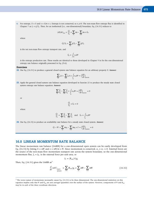
- Page 696 and 697: 16.7 Reynolds Transport Theorem 671
- Page 700 and 701: 16.9 Shock Waves 675 16.9 SHOCK WAV
- Page 702 and 703: 16.9 Shock Waves 677 and, for an id
- Page 704 and 705: 16.9 Shock Waves 679 6 5 4 S P /(m
- Page 706 and 707: 16.10 Nozzle and Diffuser Efficienc
- Page 708 and 709: 16.10 Nozzle and Diffuser Efficienc
- Page 710 and 711: Summary 685 Since for a diffuser, M
- Page 712 and 713: Problems 687 Problems (* indicates
- Page 714 and 715: 43. 0.800 lbm/s of air passes throu
- Page 716 and 717: Problems 691 A plot of this functio
- Page 718 and 719: CHAPTER 17 Thermodynamics of Biolog
- Page 720 and 721: 17.3 Thermodynamics of Biological C
- Page 722 and 723: 17.3 Thermodynamics of Biological C
- Page 724 and 725: 17.4 Energy Conversion Efficiency o
- Page 726 and 727: 17.4 Energy Conversion Efficiency o
- Page 728 and 729: 17.5 Metabolism 703 Table 17.3 Brea
- Page 730 and 731: 17.6 Thermodynamics of Nutrition an
- Page 732 and 733: 17.6 Thermodynamics of Nutrition an
- Page 734 and 735: 17.6 Thermodynamics of Nutrition an
- Page 736 and 737: 17.7 Limits to Biological Growth 71
- Page 738 and 739: 17.7 Limits to Biological Growth 71
- Page 740 and 741: 17.8 Locomotion Transport Number 71
- Page 742 and 743: 17.9 Thermodynamics of Aging and De
- Page 744 and 745: 17.9 Thermodynamics of Aging and De
- Page 746 and 747: 1/3 V most efficient = P o ρAC D S
- Page 748 and 749:
Problems 723 a. If the monster cons
- Page 750 and 751:
Problems 725 the officer asks Paul
- Page 752 and 753:
CHAPTER 18 Introduction to Statisti
- Page 754 and 755:
18.3 Kinetic Theory of Gases 729 3.
- Page 756 and 757:
U trans = 3 2 NkT (Continued ) 18.3
- Page 758 and 759:
18.4 Intermolecular Collisions 733
- Page 760 and 761:
18.5 Molecular Velocity Distributio
- Page 762 and 763:
18.5 Molecular Velocity Distributio
- Page 764 and 765:
18.6 Equipartition of Energy 739 We
- Page 766 and 767:
18.7 Introduction to Mathematical P
- Page 768 and 769:
18.7 Introduction to Mathematical P
- Page 770 and 771:
18.7 Introduction to Mathematical P
- Page 772 and 773:
18.8 Quantum Statistical Thermodyna
- Page 774 and 775:
18.9 Three Classical Quantum Statis
- Page 776 and 777:
18.11 Monatomic Maxwell-Boltzmann G
- Page 778 and 779:
18.12 Diatomic Maxwell-Boltzmann Ga
- Page 780 and 781:
18.12 Diatomic Maxwell-Boltzmann Ga
- Page 782 and 783:
18.13 Polyatomic Maxwell-Boltzmann
- Page 784 and 785:
Summary 759 In this chapter, we sum
- Page 786 and 787:
Problems 761 4. Find the temperatur
- Page 788 and 789:
CHAPTER 19 Introduction to Coupled
- Page 790 and 791:
19.3 Linear Phenomenological Equati
- Page 792 and 793:
19.4 Thermoelectric Coupling 767 Eq
- Page 794 and 795:
19.4 Thermoelectric Coupling 769 Th
- Page 796 and 797:
19.4 Thermoelectric Coupling 771 wh
- Page 798 and 799:
19.4 Thermoelectric Coupling 773 Th
- Page 800 and 801:
19.4 Thermoelectric Coupling 775 b.
- Page 802 and 803:
19.5 Thermomechanical Coupling 777
- Page 804 and 805:
19.5 Thermomechanical Coupling 779
- Page 806 and 807:
19.5 Thermomechanical Coupling 781
- Page 808 and 809:
water), it seems reasonable that li
- Page 810 and 811:
Problems 785 b. For a Knudson gas,
- Page 812 and 813:
Appendix A: Physical Constants and
- Page 814 and 815:
Appendix B: Greek and Latin Origins
- Page 816 and 817:
Appendix B 791 Table B.4 Plural End
- Page 818 and 819:
Index Page numbers followed by f in
- Page 820 and 821:
Index 795 E e (specific energy), 10
- Page 822 and 823:
Index 797 Isobaric coefficient of v
- Page 824 and 825:
Index 799 Ranque, Georges Joseph, 3
- Page 826 and 827:
Index 801 William III, King of Engl