characterization, modeling, and design of esd protection circuits

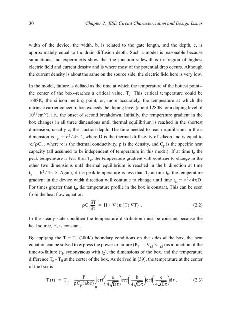
30 Chapter 2. ESD Circuit Characterization and Design Issues
width of the device, the width, b, is related to the gate length, and the depth, c, is
approximately equal to the drain diffusion depth. Such a model is reasonable because
simulations and experiments show that the junction sidewall is the region of highest
electric field and current density and is where most of the potential drop occurs. Although
the current density is about the same on the source side, the electric field here is very low.
In the model, failure is defined as the time at which the temperature of the hottest pointthe
center of the box--reaches a critical value, Tc . This critical temperature could be
1688K, the silicon melting point, or, more accurately, the temperature at which the
intrinsic carrier concentration exceeds the doping level (about 1280K for a doping level of
10 18 cm -3 ), i.e., the onset of second breakdown. Initially, the temperature gradient in the
box changes in all three dimensions until thermal equilibrium is reached in the shortest
dimension, usually c, the junction depth. The time needed to reach equilibrium in the c
dimension is tc c , where D is the thermal diffusivity of silicon and is equal to
, where κ is the thermal conductivity, ρ is the density, and Cp is the specific heat
capacity (all assumed to be independent of temperature in this model). If at time tc the
peak temperature is less than Tc , the temperature gradient will continue to change in the
other two dimensions until thermal equilibrium is reached in the b direction at time
. Again, if the peak temperature is less than Tc at time tb , the temperature
gradient in the device width direction will continue to change until time .
For times greater than ta , the temperature profile in the box is constant. This can be seen
from the heat flow equation:
2 = ⁄ 4πD
κ ⁄ ρCp tb b2 = ⁄ 4πD
ta a2 = ⁄ 4πD
∂T
ρCp∂ t
= H + ∇ ( κ ( T)
∇T)
. (2.2)
In the steady-state condition the temperature distribution must be constant because the
heat source, H, is constant.
By applying the T = T0 (300K) boundary conditions on the sides of the box, the heat
equation can be solved to express the power to failure ( Pf = Vt2 × It2) as a function of the
time-to-failure (tf , synonymous with t2 ), the dimensions of the box, and the temperature
difference Tc - T0 at the center of the box. As derived in [39], the temperature at the center
of the box is
t
P
T() t T0 ------------------------- erf⎛
a
-------------- ⎞erf⎛ b
-------------- ⎞ c
=
+
erf⎛--------------
⎞ , (2.3)
ρCp ( abc)
∫
dτ
⎝4 Dτ⎠
⎝4 Dτ⎠
⎝4 Dτ⎠
0