- Page 1:
I.S.F.A. École Doctorale Sciences
- Page 5:
If you want to be happy... ... for
- Page 9 and 10:
Table des matières Remerciements R
- Page 11 and 12:
Conclusion et annexes Conclusion et
- Page 13:
Introduction générale 1
- Page 16 and 17:
Présentation de la thèse personne
- Page 18 and 19:
Présentation de la thèse Les assu
- Page 20 and 21:
Présentation de la thèse maux, et
- Page 22 and 23:
Présentation de la thèse Figure 1
- Page 24 and 25:
Présentation de la thèse visible
- Page 26 and 27:
Présentation de la thèse Proposit
- Page 28 and 29:
Présentation de la thèse { } avec
- Page 30 and 31:
Présentation de la thèse Bibliogr
- Page 32 and 33:
Présentation de la thèse Torsten,
- Page 35 and 36:
Chapitre 1 Segmentation du risque d
- Page 37 and 38:
1.1. Modélisation CART Constructio
- Page 39 and 40:
1.1. Modélisation CART nous entend
- Page 41 and 42:
1.2. Segmentation par modèle logis
- Page 43 and 44:
1.2. Segmentation par modèle logis
- Page 45 and 46:
1.3. Illustration : application sur
- Page 47 and 48:
1.3. Illustration : application sur
- Page 49 and 50:
1.3. Illustration : application sur
- Page 51 and 52:
1.3. Illustration : application sur
- Page 53 and 54:
1.4. Conclusion Enfin cette analyse
- Page 55 and 56:
BIBLIOGRAPHIE Ruiz-Gazen, A. and Vi
- Page 57 and 58:
Chapitre 2 Crises de corrélation d
- Page 59 and 60:
2.1. Problème de la régression lo
- Page 61 and 62:
2.2. Impact de crises de corrélati
- Page 63 and 64:
2.2. Impact de crises de corrélati
- Page 65 and 66:
2.2. Impact de crises de corrélati
- Page 67 and 68:
2.2. Impact de crises de corrélati
- Page 69 and 70:
2.2. Impact de crises de corrélati
- Page 71 and 72:
2.3. Application sur un portefeuill
- Page 73 and 74:
2.3. Application sur un portefeuill
- Page 75 and 76:
2.4. Ecart entre hypothéses standa
- Page 77 and 78:
2.5. Conclusion encore considérer
- Page 79:
Deuxième partie Vers la création
- Page 82 and 83:
Chapitre 3. Mélange de régression
- Page 84 and 85:
Chapitre 3. Mélange de régression
- Page 86 and 87: Chapitre 3. Mélange de régression
- Page 88 and 89: Chapitre 3. Mélange de régression
- Page 90 and 91: Chapitre 3. Mélange de régression
- Page 92 and 93: Chapitre 3. Mélange de régression
- Page 94 and 95: Chapitre 3. Mélange de régression
- Page 96 and 97: Chapitre 3. Mélange de régression
- Page 98 and 99: Chapitre 3. Mélange de régression
- Page 100 and 101: Chapitre 3. Mélange de régression
- Page 102 and 103: Chapitre 3. Mélange de régression
- Page 104 and 105: Chapitre 3. Mélange de régression
- Page 106 and 107: Chapitre 3. Mélange de régression
- Page 108 and 109: Chapitre 3. Mélange de régression
- Page 110 and 111: Chapitre 3. Mélange de régression
- Page 112 and 113: Chapitre 3. Mélange de régression
- Page 114 and 115: Chapitre 3. Mélange de régression
- Page 116 and 117: Chapitre 4. Sélection de mélange
- Page 118 and 119: Chapitre 4. Sélection de mélange
- Page 120 and 121: Chapitre 4. Sélection de mélange
- Page 122 and 123: Chapitre 4. Sélection de mélange
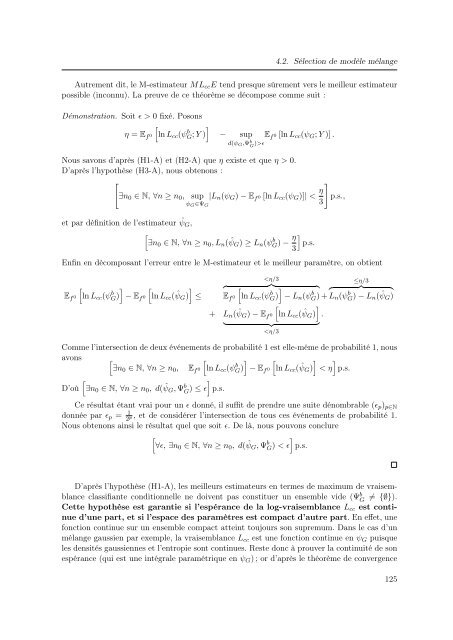
- Page 124 and 125: Chapitre 4. Sélection de mélange
- Page 126 and 127: Chapitre 4. Sélection de mélange
- Page 128 and 129: Chapitre 4. Sélection de mélange
- Page 130 and 131: Chapitre 4. Sélection de mélange
- Page 132 and 133: Chapitre 4. Sélection de mélange
- Page 134 and 135: Chapitre 4. Sélection de mélange
- Page 138 and 139: Chapitre 4. Sélection de mélange
- Page 140 and 141: Chapitre 4. Sélection de mélange
- Page 142 and 143: Chapitre 4. Sélection de mélange
- Page 144 and 145: Chapitre 4. Sélection de mélange
- Page 146 and 147: Chapitre 4. Sélection de mélange
- Page 148 and 149: Chapitre 4. Sélection de mélange
- Page 150 and 151: Chapitre 4. Sélection de mélange
- Page 152 and 153: Chapitre 4. Sélection de mélange
- Page 154 and 155: Chapitre 4. Sélection de mélange
- Page 156 and 157: Chapitre 4. Sélection de mélange
- Page 158 and 159: Chapitre 4. Sélection de mélange
- Page 160 and 161: Chapitre 4. Sélection de mélange
- Page 162 and 163: Chapitre 4. Sélection de mélange
- Page 164 and 165: Chapitre 4. Sélection de mélange
- Page 166 and 167: Chapitre 4. Sélection de mélange
- Page 168 and 169: Chapitre 4. Sélection de mélange
- Page 170 and 171: Chapitre 4. Sélection de mélange
- Page 172 and 173: Chapitre 4. Sélection de mélange
- Page 174 and 175: Chapitre 4. Sélection de mélange
- Page 176 and 177: Chapitre 4. Sélection de mélange
- Page 178 and 179: Chapitre 4. Sélection de mélange
- Page 180 and 181: Chapitre 4. Sélection de mélange
- Page 182 and 183: Chapitre 4. Sélection de mélange
- Page 184 and 185: Chapitre 4. Sélection de mélange
- Page 186 and 187:
Chapitre 4. Sélection de mélange
- Page 189 and 190:
Conclusion et perspectives Cette é
- Page 191 and 192:
BIBLIOGRAPHIE Bibliographie Akaike,
- Page 193 and 194:
BIBLIOGRAPHIE Doob, J. (1934), ‘P
- Page 195 and 196:
BIBLIOGRAPHIE Loisel, S. (2008),
- Page 197 and 198:
BIBLIOGRAPHIE Schlattmann, P. (2003
- Page 199 and 200:
Annexe A Articles de presse Figure
- Page 201 and 202:
Annexe B Méthodes de segmentation
- Page 203 and 204:
B.1.3 Plus loin dans la théorie de
- Page 205 and 206:
B.1. Méthode CART Pénalisation de
- Page 207 and 208:
B.2. La régression logistique Algo
- Page 209 and 210:
B.2. La régression logistique et e
- Page 211 and 212:
Annexe C Résultats des mélanges d
- Page 213 and 214:
C.2. Famille de produits Ahorro Fig
- Page 215 and 216:
C.2. Famille de produits Ahorro C.2
- Page 217 and 218:
C.3. Famille de produits Unit-Link
- Page 219 and 220:
C.3. Famille de produits Unit-Link
- Page 221 and 222:
C.4. Famille de produits Index-Link
- Page 223 and 224:
C.4. Famille de produits Index-Link
- Page 225 and 226:
C.5. Famille de produits Universal
- Page 227 and 228:
C.5. Famille de produits Universal
- Page 229 and 230:
C.6. Famille de produits Pure Savin
- Page 231 and 232:
C.6. Famille de produits Pure Savin
- Page 233 and 234:
C.7. Famille de produits “Structu
- Page 235 and 236:
C.7. Famille de produits “Structu
- Page 237 and 238:
Annexe D Espace des paramètres des
- Page 239 and 240:
D.1. Mélange de régressions liné
- Page 241 and 242:
D.3 Mélange de régressions logist
- Page 243 and 244:
Calcul de la limite : lim log L cc(
- Page 245 and 246:
D.5. Mélange d’Inverses Gaussien
- Page 247 and 248:
Annexe E Outil informatique - RExce
- Page 249 and 250:
Figure E.2 - Exemple d’interface
- Page 251 and 252:
Figure E.4 - Génération des résu
- Page 253 and 254:
Figure E.6 - Exposition des résult