Mélanges de GLMs et nombre de composantes : application ... - Scor
Mélanges de GLMs et nombre de composantes : application ... - Scor
Mélanges de GLMs et nombre de composantes : application ... - Scor

Create successful ePaper yourself
Turn your PDF publications into a flip-book with our unique Google optimized e-Paper software.
Chapitre 2. Crises <strong>de</strong> corrélation <strong>de</strong>s comportements<br />
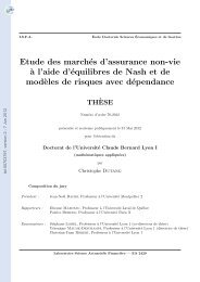
Figure 2.8 – Ecart relatif (en %) <strong>de</strong>s V aR versus p 0 <strong>et</strong> p.<br />
70<br />
60<br />
50<br />
1.0<br />
40<br />
z<br />
60<br />
40<br />
20<br />
0.8<br />
0.6<br />
Correlation 0.4 (p0)<br />
30<br />
20<br />
0<br />
0.0 0.2 0.4 0.6 0.8 0.0<br />
1.0<br />
0.2<br />
10<br />
Indiv. surren<strong>de</strong>r prob.(p)<br />
0<br />
La taille <strong>de</strong> la compagnie pourrait également être un facteur-clef : pour tester son impact,<br />
nous avons simulé les écarts <strong>de</strong> capital économique (EC) lié à la V aR pour une probabilité<br />
annuelle moyenne <strong>de</strong> rachat réaliste <strong>de</strong> 8,08 % (BE pour best-estimate dans le tableau 2.4) <strong>et</strong><br />
une corrélation passant <strong>de</strong> 0 % à 50 %. Etudier les écarts <strong>de</strong> capitaux économiques revient<br />
à étudier les écarts <strong>de</strong> V aR (voir graphe 2.7). Certaines compagnies d’assurance pourraient<br />
penser que leur taille leur évite <strong>de</strong>s scénarios catastrophiques grâce à l’eff<strong>et</strong> <strong>de</strong> la mutualisation.<br />
L’analyse du tableau 2.4 démontre que le <strong>nombre</strong> d’assurés en portefeuille n’a pas <strong>de</strong> forte<br />
influence sur le calcul <strong>de</strong>s marges <strong>de</strong> risque. En eff<strong>et</strong>, la différence <strong>de</strong> capital économique ∆EC<br />
nécessaire baisse <strong>de</strong> manière dérisoire, même en passant <strong>de</strong> 5 000 à 500 000 assurés ! Une<br />
<strong>application</strong> complète sur un exemple <strong>de</strong> produit est menée dans Loisel and Milhaud (2011).<br />
Taille portefeuille BE EC (V aR99.5% Normale ) Corrélation EC (V aRBimodale<br />
99.5%<br />
) ∆EC<br />
P<strong>et</strong>ite : p 0 = 0.05 6.26% 4.5%<br />
5000 8.08% 1.76% p 0 = 0.2 20.42% 18.66%<br />
assurés (p 0 = 0) (p 0 = 0) p 0 = 0.5 48.54% 46.78%<br />
Moyenne : p 0 = 0.05 5.1% 4.59%<br />
50 000 8.08% 0.51% p 0 = 0.2 19.01% 18.5%<br />
assurés (p 0 = 0) (p 0 = 0) p 0 = 0.5 46.63% 46.12%<br />
Gran<strong>de</strong> : p 0 = 0.05 4.73% 4.59%<br />
500 000 8.08% 0.1426% p 0 = 0.2 18.56% 18.41%<br />
assurés (p 0 = 0) (p 0 = 0) p 0 = 0.5 46.16% 46.01%<br />
Table 2.1 – Impact <strong>de</strong> la taille du portefeuille sur la V aR (100 000 simulations).<br />
58