Mélanges de GLMs et nombre de composantes : application ... - Scor
Mélanges de GLMs et nombre de composantes : application ... - Scor
Mélanges de GLMs et nombre de composantes : application ... - Scor

Create successful ePaper yourself
Turn your PDF publications into a flip-book with our unique Google optimized e-Paper software.
Annexe C. Résultats <strong>de</strong>s mélanges <strong>de</strong> Logit<br />
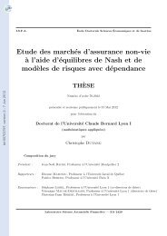
Figure C.25 – Coefficients <strong>de</strong> régression <strong>de</strong>s <strong>composantes</strong>, produits Universal Savings.<br />
−10 −5 0<br />
end.month04<br />
end.month07<br />
end.month10<br />
duration.rangelow.duration<br />
duration.rangemiddle.duration<br />
un<strong>de</strong>rwritingAge.range2<br />
un<strong>de</strong>rwritingAge.range3<br />
dist.channelcommercial.intensive<br />
dist.channelnon−available<br />
(Intercept)<br />
fa.rangelow.face.amount<br />
fa.rangemiddle.face.amount<br />
Comp. 1<br />
Comp. 4<br />
−10 −5 0<br />
Comp. 2 Comp. 3<br />
Comp. 5<br />
end.month04<br />
end.month07<br />
end.month10<br />
duration.rangelow.duration<br />
duration.rangemiddle.duration<br />
un<strong>de</strong>rwritingAge.range2<br />
un<strong>de</strong>rwritingAge.range3<br />
dist.channelcommercial.intensive<br />
dist.channelnon−available<br />
(Intercept)<br />
fa.rangelow.face.amount<br />
fa.rangemiddle.face.amount<br />
C.6 Famille <strong>de</strong> produits Pure Savings<br />
C.6.1<br />
Analyse <strong>de</strong>scriptive<br />
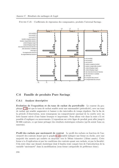
Evolution <strong>de</strong> l’exposition <strong>et</strong> du taux <strong>de</strong> rachat du portefeuille Le constat du graphique<br />
C.26 est que le taux <strong>de</strong> rachat semble avoir une saisonnalité (périodicité), avec un taux<br />
<strong>de</strong> rachat qui semble augmenter <strong>et</strong> baisser à <strong>de</strong>s intervalles <strong>de</strong> temps réguliers. Sur la fin <strong>de</strong><br />
la pério<strong>de</strong> d’observation, nous remarquons un comportement anormal <strong>de</strong> la courbe avec un<br />
forte hausse suivie d’une baisse brusque <strong>et</strong> importante. Nous allons voir dans la suite s’il est<br />
possible d’expliquer ces mouvements. L’exposition sur c<strong>et</strong>te ligne <strong>de</strong> produit peut aller jusqu’à<br />
80 000 contrats, ce qui laisse présager <strong>de</strong>s résultats statistiques robustes (qu’ils soient bons ou<br />
mauvais).<br />
Profil <strong>de</strong>s rachats par ancienn<strong>et</strong>é <strong>de</strong> contrat Le profil <strong>de</strong>s rachats en fonction <strong>de</strong> l’ancienn<strong>et</strong>é<br />
<strong>de</strong>s contrats donné par le graphe C.27 semble indiquer une forme en cloche, avec une<br />
majorité <strong>de</strong>s assurés qui rachète en moyenne vers le 50ème trimestre (13ème année). C<strong>et</strong>te<br />
forme n’a d’explication ni par les conditions <strong>de</strong>s contrats quant aux rachats, ni par la fiscalité.<br />
Cela reste donc une donnée statistique dont il faudra tenir compte lors <strong>de</strong> l’introduction <strong>de</strong> la<br />
variable “ancienn<strong>et</strong>é” dans la modélisation (sous forme catégorielle <strong>de</strong> préférence donc).<br />
216