Вычислительная математика - ИСЭМ СО РАН

The region is the intersection of three parts which are outside of both black, grey, and light-grey regions.
We notice that at Figure 2, the stability region is quite similar to the A(α)-stable stable methods.
5. Numerical Results
We will apply the block-type method to one nonstiff and one stiff equation. For the nonstiff equation,
the system of equation is given as the following
y ′ 1 = y 2y 3
y ′ 2 = −y 1y 3
y ′ 3 = −0.51y 1y 2
with
y 1 (0) = 0
y 2 (0) = 1
y 3 (0) = 1
(9)
We apply three numerical schemes implicitly, the first one is to apply formula Eq. (3) by Newton
iteration, the second is applying a Block formula (Equation (7) by Newton iteration, and the last one is
solved by a standard method ode45 from MATLAB. A fixed stepsize h = 5×10 −2 were used at scheme
1 and 2, and variable stepsize strategy scheme 3 was implemented, and their numerical solutions are
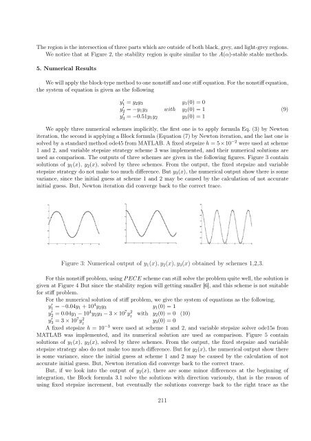
used as comparison. The outputs of three schemes are given in the following figures. Figure 3 contain
solutions of y 1 (x), y 2 (x), solved by three schemes. From the output, the fixed stepsize and variable
stepsize strategy do not make too much difference. But y 3 (x), the numerical output show there is some
variance, since the initial guess at scheme 1 and 2 may be caused by the calculation of not accurate
initial guess. But, Newton iteration did converge back to the correct trace.
Figure 3: Numerical output of y 1 (x), y 2 (x), y 3 (x) obtained by schemes 1,2,3.
For this nonstiff problem, using P ECE scheme can still solve the problem quite well, the solution is
given at Figure 4 But since the stability region will getting smaller [6], and this scheme is not suitable
for stiff problem.
For the numerical solution of stiff problem, we give the system of equations as the following,
y 1 ′ = −0.04y 1 + 10 4 y 2 y 3
y 2 ′ = 0.04y 1 − 10 4 y 2 y 3 − 3 × 10 7 y 2 2
y 3 ′ = 3 × 107 y 2 2
with
y 1 (0) = 1
y 2 (0) = 0
y 3 (0) = 0
A fixed stepsize h = 10 −3 were used at scheme 1 and 2, and variable stepsize solver ode15s from
MATLAB was implemented, and its numerical solution are used as comparison. Figure 5 contain
solutions of y 1 (x), y 2 (x), solved by three schemes. From the output, the fixed stepsize and variable
stepsize strategy also do not make too much difference. But for y 2 (x), the numerical output show there
is some variance, since the initial guess at scheme 1 and 2 may be caused by the calculation of not
accurate initial guess. But, Newton iteration did converge back to the correct trace.
But, if we look into the output of y 2 (x), there are some minor differences at the beginning of
integration, the Block formula 3.1 solve the solutions with direction variously, that is the reason of
using fixed stepsize increment, but eventually the solutions converge back to the right trace as the
211
(10)