Вычислительная математика - ИСЭМ СО РАН

More documents

Recommendations

Info

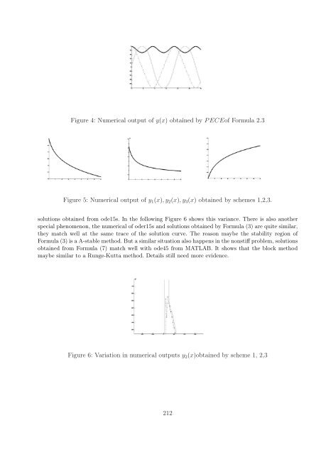
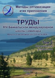
The region is the intersection of three parts which are outside of both black, grey, and light-grey regions. We notice that at Figure 2, the stability region is quite similar to the A(α)-stable stable methods. 5. Numerical Results We will apply the block-type method to one nonstiff and one stiff equation. For the nonstiff equation, the system of equation is given as the following y ′ 1 = y 2y 3 y ′ 2 = −y 1y 3 y ′ 3 = −0.51y 1y 2 with y 1 (0) = 0 y 2 (0) = 1 y 3 (0) = 1 (9) We apply three numerical schemes implicitly, the first one is to apply formula Eq. (3) by Newton iteration, the second is applying a Block formula (Equation (7) by Newton iteration, and the last one is solved by a standard method ode45 from MATLAB. A fixed stepsize h = 5×10 −2 were used at scheme 1 and 2, and variable stepsize strategy scheme 3 was implemented, and their numerical solutions are used as comparison. The outputs of three schemes are given in the following figures. Figure 3 contain solutions of y 1 (x), y 2 (x), solved by three schemes. From the output, the fixed stepsize and variable stepsize strategy do not make too much difference. But y 3 (x), the numerical output show there is some variance, since the initial guess at scheme 1 and 2 may be caused by the calculation of not accurate initial guess. But, Newton iteration did converge back to the correct trace. Figure 3: Numerical output of y 1 (x), y 2 (x), y 3 (x) obtained by schemes 1,2,3. For this nonstiff problem, using P ECE scheme can still solve the problem quite well, the solution is given at Figure 4 But since the stability region will getting smaller [6], and this scheme is not suitable for stiff problem. For the numerical solution of stiff problem, we give the system of equations as the following, y 1 ′ = −0.04y 1 + 10 4 y 2 y 3 y 2 ′ = 0.04y 1 − 10 4 y 2 y 3 − 3 × 10 7 y 2 2 y 3 ′ = 3 × 107 y 2 2 with y 1 (0) = 1 y 2 (0) = 0 y 3 (0) = 0 A fixed stepsize h = 10 −3 were used at scheme 1 and 2, and variable stepsize solver ode15s from MATLAB was implemented, and its numerical solution are used as comparison. Figure 5 contain solutions of y 1 (x), y 2 (x), solved by three schemes. From the output, the fixed stepsize and variable stepsize strategy also do not make too much difference. But for y 2 (x), the numerical output show there is some variance, since the initial guess at scheme 1 and 2 may be caused by the calculation of not accurate initial guess. But, Newton iteration did converge back to the correct trace. But, if we look into the output of y 2 (x), there are some minor differences at the beginning of integration, the Block formula 3.1 solve the solutions with direction variously, that is the reason of using fixed stepsize increment, but eventually the solutions converge back to the right trace as the 211 (10)
Figure 4: Numerical output of y(x) obtained by P ECEof Formula 2.3 Figure 5: Numerical output of y 1 (x), y 2 (x), y 3 (x) obtained by schemes 1,2,3. solutions obtained from ode15s. In the following Figure 6 shows this variance. There is also another special phenomenon, the numerical of oder15s and solutions obtained by Formula (3) are quite similar, they match well at the same trace of the solution curve. The reason maybe the stability region of Formula (3) is a A-stable method. But a similar situation also happens in the nonstiff problem, solutions obtained from Formula (7) match well with ode45 from MATLAB. It shows that the block method maybe similar to a Runge-Kutta method. Details still need more evidence. Figure 6: Variation in numerical outputs y 2 (x)obtained by scheme 1, 2,3 212
Page 2 and 3:
Российская академи
Page 4 and 5:
Russian Academy of Sciences (RAS) R
Page 6 and 7:
СОДЕРЖАНИЕ Абдулли
Page 8 and 9:
ОБЛАСТИ ПРИТЯЖЕНИЯ
Page 10 and 11:
W2,0 S = {x ∈ W1,0 V : f 1 (x)
Page 12 and 13:
при W 0 ≠ ∅ и f 1 W 0 ⊂ G
Page 14 and 15:
Список литературы [
Page 16 and 17:
О ДВУХ ПОДХОДАХ К П
Page 18 and 19:
2. Ниже рассматрива
Page 20 and 21:
то Случай N = 2, L 1 > 0, L
Page 22 and 23:
СРАВНЕНИЕ АЛГОРИТМ
Page 24 and 25:
Совершенно другой
Page 26 and 27:
а) б) 1 0.8 0.6 0.4 0.2 0 −0.2
Page 28 and 29:
ОБ ОДНОМ КЛАССЕ ВЫР
Page 30 and 31:
4. Пучок матриц λA(t, x
Page 32 and 33:
Page 34 and 35:
Определение 1. Матр
Page 36 and 37:
Достаточные услови
Page 38 and 39:
Список (17) содержит
Page 40 and 41:
[8] B.E.Cain Real, 3 × 3 D-stable
Page 42 and 43:
12 2 2 3 2 4 2 5 2 = −∆ 2 5 −
Page 44 and 45:
О СВОЙСТВАХ КОНЕЧН
Page 46 and 47:
Из определения 2 сл
Page 48 and 49:
где E ρn ( + λ(E ρn − AA
Page 50 and 51:
где c 1 = (E−A − 0 A 0 )c
Page 52 and 53:
( ) ( ) ( ) x2 − x F 1 (x) = 2 1
Page 54 and 55:
дополнение. Тогда о
Page 56 and 57:
6. Заключение Иссле
Page 58 and 59:
ON THE PROPERTIES OF FINITE-DIMENSI
Page 60 and 61:
где dσ - элемент пло
Page 62 and 63:
Таким образом, сист
Page 64 and 65:
т.е. P - это соприкас
Page 66 and 67:
в которых равномер
Page 68 and 69:
абсолютные значени
Page 70 and 71:
МЕТОД НОРМАЛЬНЫХ С
Page 72 and 73:
значения изображен
Page 74 and 75:
матрицей Грама кан
Page 76 and 77:
узлов на каждой. По
Page 78 and 79:
МЕТОДЫ ИНТЕГРИРОВА
Page 80 and 81:
водить теоретическ
Page 82 and 83:
циально-алгебраиче
Page 84 and 85:
К системе (9) примен
Page 86 and 87:
[4] В.В. Дикуcap. Метод
Page 88 and 89:
где I(x(t)) = ∫ T t 0 a t−t
Page 90 and 91:
Заметим, что (6)-(13) -
Page 92 and 93:
1.4 1.2 1 y 0.8 0.6 0.4 0.2 0 1 2 3
Page 94 and 95:
Потребуем Дифферен
Page 96 and 97:
ON DEVELOPING SYSTEMS MODELS I.V. K
Page 98 and 99:
очень затруднитель
Page 100 and 101:
Теорема 1.3. Пусть пу
Page 102 and 103:
Далее по формулам,
Page 104 and 105:
ФУНДАМЕНТАЛЬНАЯ ОП
Page 106 and 107:
Покажем единственн
Page 108 and 109:
Для завершения док
Page 110 and 111:
где U Nν (t) = 1 ∫ 2πi γ (
Page 112 and 113:
ЧИСЛЕННОЕ РЕШЕНИЕ
Page 114 and 115:
Количественные и к
Page 116 and 117:
Рис. 1: Изменение ск
Page 118 and 119:
THE NUMERICAL SOLUTION FOR ONE PROB
Page 120 and 121:
Определение 2. [1] Со
Page 122 and 123:
Далее нетрудно сос
Page 124 and 125:
Далее подействуем
Page 126 and 127:
Page 128 and 129:
поле описывается у
Page 130 and 131:
∑ ∫ (u kl − u 0 kl) (k,l)∈D
Page 132 and 133:
5. Численный экспер
Page 134 and 135:
к тому, что первый п
Page 136 and 137:
умноженную на любо
Page 138 and 139:
1) p < 2 √ r; 2) p 2 √ r. В
Page 140 and 141:
V 1 (z) , доставляющие
Page 142 and 143:
[8] Курош А.Г. Курс вы
Page 144 and 145:
порядка точности п
Page 146 and 147:
где k 1 и k 2 вычисляю
Page 148 and 149:
меньше последнего
Page 150 and 151:
жесткая для явных м
Page 152 and 153:
AN ALGORITHM BASED ON THE SECOND OR
Page 154 and 155:
распознавание, мин
Page 156 and 157:
Пусть A i (δ) - интерв
Page 158 and 159:
как алгоритмы рабо
Page 160 and 161:
где оператор Φ(V, λ)
Page 162 and 163: Подставляя получен
Page 164 and 165: IMPLICIT FUNCTION THEOREM IN SECTOR
Page 166 and 167: локальной выборки,
Page 168 and 169: ˜z (1) k на опорном из
Page 170 and 171: где g - отношение си
Page 172 and 173: [4] Самойлов М. Ю. Опт
Page 174 and 175: K(t) = A + ∫ t 0 k(s)ds. Теор
Page 176 and 177: при i = 1, . . . , n. По та
Page 178 and 179: Из представления ˜B
Page 180 and 181: поэтому условия со
Page 182 and 183: О СВОЙСТВАХ ВЫРОЖД
Page 184 and 185: Продифференцируем
Page 186 and 187: [3] Булатов М.В. Числ
Page 188 and 189: реальных постаново
Page 190 and 191: Обычные интервалы
Page 192 and 193: 3. Вычисление форма
Page 194 and 195: Но rad (GH) |G| · rad H для
Page 196 and 197: YET ANOTHER VERSION OF FORMAL APPRO
Page 198 and 199: специального вида (
Page 200 and 201: s k = 0, при k < 0 или k > n.
Page 202 and 203: Шаг 2. Найти (оценит
Page 204 and 205: THE TOLERABLE SOLUTION SET OF INTER
Page 206 and 207: Obviously function F x (η) is posi
Page 208 and 209: О НЕПРЕРЫВНОМ РЕШЕ
Page 210 and 211: Forh ∈ (0, h 0 ], letx k = a + kh
Page 214 and 215: 6. Conclusions. A block-type family
Page 216: ТРУДЫ секции "Вычис
show all

Вычислительная математика - ИСЭМ СО РАН

Create successful ePaper yourself

Delete template?

Save as template?