- Page 2:
Research Methods in Education This
- Page 5 and 6:
First published 2007 by Routledge 2
- Page 8 and 9:
Contents List of boxes xiii Acknowl
- Page 10 and 11:
CONTENTS ix Searching for research
- Page 12:
CONTENTS xi Part 5 Data analysis 22
- Page 15 and 16:
xiv BOXES 13.1 Independent and depe
- Page 17 and 18:
xvi BOXES 24.54 Frequencies and per
- Page 19 and 20:
xviii ACKNOWLEDGEMENTS Springer,for
- Page 21 and 22:
2 INTRODUCTION Package for the Soci
- Page 24 and 25:
1 The nature of inquiry - Setting t
- Page 26 and 27:
TWO CONCEPTIONS OF SOCIAL REALITY 7
- Page 28 and 29:
POSITIVISM 9 Box 1.1 The subjective
- Page 30 and 31:
THE ASSUMPTIONS AND NATURE OF SCIEN
- Page 32 and 33:
THE ASSUMPTIONS AND NATURE OF SCIEN
- Page 34 and 35:
THE SCIENTIFIC METHOD 15 an educate
- Page 36 and 37:
CRITICISMS OF POSITIVISM AND THE SC
- Page 38 and 39:
ALTERNATIVES TO POSITIVISTIC SOCIAL
- Page 40 and 41:
A QUESTION OF TERMINOLOGY: THE NORM
- Page 42 and 43:
PHENOMENOLOGY, ETHNOMETHODOLOGY AND
- Page 44 and 45:
CRITICISMS OF THE NATURALISTIC AND
- Page 46 and 47:
CRITICAL THEORY AND CRITICAL EDUCAT
- Page 48 and 49:
CRITICISMS OF APPROACHES FROM CRITI
- Page 50 and 51:
CRITICAL THEORY AND CURRICULUM RESE
- Page 52 and 53:
THE EMERGING PARADIGM OF COMPLEXITY
- Page 54 and 55:
FEMINIST RESEARCH 35 deconstructin
- Page 56 and 57:
FEMINIST RESEARCH 37 respecting d
- Page 58 and 59:
FEMINIST RESEARCH 39 Research must
- Page 60 and 61:
RESEARCH AND EVALUATION 41 particul
- Page 62 and 63:
RESEARCH AND EVALUATION 43 The age
- Page 64 and 65:
RESEARCH AND EVALUATION 45 to exten
- Page 66 and 67:
METHODS AND METHODOLOGY 47 too easi
- Page 68:
Part Two Planning educational resea
- Page 71 and 72:
52 THE ETHICS OF EDUCATIONAL AND SO
- Page 73 and 74:
54 THE ETHICS OF EDUCATIONAL AND SO
- Page 75 and 76: 56 THE ETHICS OF EDUCATIONAL AND SO
- Page 77 and 78: 58 THE ETHICS OF EDUCATIONAL AND SO
- Page 79 and 80: 60 THE ETHICS OF EDUCATIONAL AND SO
- Page 81 and 82: 62 THE ETHICS OF EDUCATIONAL AND SO
- Page 83 and 84: 64 THE ETHICS OF EDUCATIONAL AND SO
- Page 85 and 86: 66 THE ETHICS OF EDUCATIONAL AND SO
- Page 87 and 88: 68 THE ETHICS OF EDUCATIONAL AND SO
- Page 89 and 90: 70 THE ETHICS OF EDUCATIONAL AND SO
- Page 91 and 92: 72 THE ETHICS OF EDUCATIONAL AND SO
- Page 93 and 94: 74 THE ETHICS OF EDUCATIONAL AND SO
- Page 95 and 96: 76 THE ETHICS OF EDUCATIONAL AND SO
- Page 97 and 98: 3 Planning educational research Int
- Page 99 and 100: 80 PLANNING EDUCATIONAL RESEARCH t
- Page 101 and 102: 82 PLANNING EDUCATIONAL RESEARCH de
- Page 103 and 104: 84 PLANNING EDUCATIONAL RESEARCH Bo
- Page 105 and 106: 86 PLANNING EDUCATIONAL RESEARCH Bo
- Page 107 and 108: 88 PLANNING EDUCATIONAL RESEARCH Bo
- Page 109 and 110: 90 PLANNING EDUCATIONAL RESEARCH Bo
- Page 111 and 112: 92 PLANNING EDUCATIONAL RESEARCH Bo
- Page 113 and 114: 94 PLANNING EDUCATIONAL RESEARCH Bo
- Page 115 and 116: 96 PLANNING EDUCATIONAL RESEARCH Or
- Page 117 and 118: 98 PLANNING EDUCATIONAL RESEARCH Pa
- Page 119 and 120: 4 Sampling Introduction The quality
- Page 121 and 122: 102 SAMPLING sample of 200 might be
- Page 123 and 124: 104 SAMPLING Box 4.1 Sample size, c
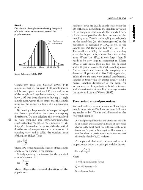
- Page 125: 106 SAMPLING would be insufficient
- Page 129 and 130: 110 SAMPLING school governors, scho
- Page 131 and 132: 112 SAMPLING terms of sex, a random
- Page 133 and 134: 114 SAMPLING the required sample si
- Page 135 and 136: 116 SAMPLING Snowball sampling In s
- Page 137 and 138: 118 SAMPLING the kind of sample (d
- Page 139 and 140: 120 SENSITIVE EDUCATIONAL RESEARCH
- Page 141 and 142: 122 SENSITIVE EDUCATIONAL RESEARCH
- Page 143 and 144: 124 SENSITIVE EDUCATIONAL RESEARCH
- Page 145 and 146: 126 SENSITIVE EDUCATIONAL RESEARCH
- Page 147 and 148: 128 SENSITIVE EDUCATIONAL RESEARCH
- Page 149 and 150: 130 SENSITIVE EDUCATIONAL RESEARCH
- Page 151 and 152: 132 SENSITIVE EDUCATIONAL RESEARCH
- Page 153 and 154: 134 VALIDITY AND RELIABILITY It is
- Page 155 and 156: 136 VALIDITY AND RELIABILITY using
- Page 157 and 158: 138 VALIDITY AND RELIABILITY includ
- Page 159 and 160: 140 VALIDITY AND RELIABILITY leadin
- Page 161 and 162: 142 VALIDITY AND RELIABILITY social
- Page 163 and 164: 144 VALIDITY AND RELIABILITY this i
- Page 165 and 166: 146 VALIDITY AND RELIABILITY prese
- Page 167 and 168: 148 VALIDITY AND RELIABILITY by ass
- Page 169 and 170: 150 VALIDITY AND RELIABILITY Validi
- Page 171 and 172: 152 VALIDITY AND RELIABILITY typica
- Page 173 and 174: 154 VALIDITY AND RELIABILITY people
- Page 175 and 176: 156 VALIDITY AND RELIABILITY
- Page 177 and 178:
158 VALIDITY AND RELIABILITY sensit
- Page 179 and 180:
160 VALIDITY AND RELIABILITY certif
- Page 181 and 182:
162 VALIDITY AND RELIABILITY how m
- Page 183 and 184:
164 VALIDITY AND RELIABILITY operat
- Page 186 and 187:
7 Naturalistic and ethnographic res
- Page 188 and 189:
ELEMENTS OF NATURALISTIC INQUIRY 16
- Page 190 and 191:
PLANNING NATURALISTIC RESEARCH 171
- Page 192 and 193:
PLANNING NATURALISTIC RESEARCH 173
- Page 194 and 195:
PLANNING NATURALISTIC RESEARCH 175
- Page 196 and 197:
PLANNING NATURALISTIC RESEARCH 177
- Page 198 and 199:
PLANNING NATURALISTIC RESEARCH 179
- Page 200 and 201:
PLANNING NATURALISTIC RESEARCH 181
- Page 202 and 203:
PLANNING NATURALISTIC RESEARCH 183
- Page 204 and 205:
PLANNING NATURALISTIC RESEARCH 185
- Page 206 and 207:
CRITICAL ETHNOGRAPHY 187 Relatio
- Page 208 and 209:
SOME PROBLEMS WITH ETHNOGRAPHIC AND
- Page 210 and 211:
8 Historical and documentary resear
- Page 212 and 213:
DATA COLLECTION 193 One can see fro
- Page 214 and 215:
WRITING THE RESEARCH REPORT 195 Ext
- Page 216 and 217:
THE USE OF QUANTITATIVE METHODS 197
- Page 218 and 219:
LIFE HISTORIES 199 Box 8.2 Atypolog
- Page 220 and 221:
DOCUMENTARY RESEARCH 201 Documentar
- Page 222 and 223:
DOCUMENTARY RESEARCH 203 What are
- Page 224 and 225:
9 Surveys, longitudinal, cross-sect
- Page 226 and 227:
SOME PRELIMINARY CONSIDERATIONS 207
- Page 228 and 229:
PLANNING A SURVEY 209 structured or
- Page 230 and 231:
LONGITUDINAL, CROSS-SECTIONAL AND T
- Page 232 and 233:
LONGITUDINAL, CROSS-SECTIONAL AND T
- Page 234 and 235:
STRENGTHS AND WEAKNESSES OF LONGITU
- Page 236 and 237:
STRENGTHS AND WEAKNESSES OF LONGITU
- Page 238 and 239:
POSTAL, INTERVIEW AND TELEPHONE SUR
- Page 240 and 241:
POSTAL, INTERVIEW AND TELEPHONE SUR
- Page 242 and 243:
POSTAL, INTERVIEW AND TELEPHONE SUR
- Page 244 and 245:
EVENT HISTORY ANALYSIS 225 may be p
- Page 246 and 247:
INTERNET-BASED SURVEYS 227 packages
- Page 248 and 249:
INTERNET-BASED SURVEYS 229 instruc
- Page 250 and 251:
INTERNET-BASED SURVEYS 231 Box 10.1
- Page 252 and 253:
INTERNET-BASED SURVEYS 233 Box 10.1
- Page 254 and 255:
INTERNET-BASED SURVEYS 235 Box 10.1
- Page 256 and 257:
INTERNET-BASED SURVEYS 237 Witte et
- Page 258 and 259:
INTERNET-BASED EXPERIMENTS 239 requ
- Page 260 and 261:
INTERNET-BASED INTERVIEWS 241 ‘ne
- Page 262 and 263:
SEARCHING FOR RESEARCH MATERIALS ON
- Page 264 and 265:
COMPUTER SIMULATIONS 245 autho
- Page 266 and 267:
COMPUTER SIMULATIONS 247 computer s
- Page 268 and 269:
COMPUTER SIMULATIONS 249 On the oth
- Page 270 and 271:
GEOGRAPHICAL INFORMATION SYSTEMS 25
- Page 272 and 273:
11 Case studies What is a case stud
- Page 274 and 275:
WHAT IS A CASE STUDY 255 (providing
- Page 276 and 277:
WHAT IS A CASE STUDY 257 argue that
- Page 278 and 279:
EXAMPLES OF KINDS OF CASE STUDY 259
- Page 280 and 281:
PLANNING A CASE STUDY 261 accounts
- Page 282 and 283:
CONCLUSION 263 In the narrativ
- Page 284 and 285:
CO-RELATIONAL AND CRITERION GROUPS
- Page 286 and 287:
CHARACTERISTICS OF EX POST FACTO RE
- Page 288 and 289:
DESIGNING AN EX POST FACTO INVESTIG
- Page 290 and 291:
PROCEDURES IN EX POST FACTO RESEARC
- Page 292 and 293:
INTRODUCTION 273 Box 13.1 Independe
- Page 294 and 295:
TRUE EXPERIMENTAL DESIGNS 275 motor
- Page 296 and 297:
TRUE EXPERIMENTAL DESIGNS 277 2 Sub
- Page 298 and 299:
TRUE EXPERIMENTAL DESIGNS 279 textb
- Page 300 and 301:
TRUE EXPERIMENTAL DESIGNS 281 Facto
- Page 302 and 303:
A QUASI-EXPERIMENTAL DESIGN: THE NO
- Page 304 and 305:
PROCEDURES IN CONDUCTING EXPERIMENT
- Page 306 and 307:
EXAMPLES FROM EDUCATIONAL RESEARCH
- Page 308 and 309:
EVIDENCE-BASED EDUCATIONAL RESEARCH
- Page 310 and 311:
EVIDENCE-BASED EDUCATIONAL RESEARCH
- Page 312 and 313:
EVIDENCE-BASED EDUCATIONAL RESEARCH
- Page 314 and 315:
EVIDENCE-BASED EDUCATIONAL RESEARCH
- Page 316 and 317:
14 Action research Introduction Act
- Page 318 and 319:
PRINCIPLES AND CHARACTERISTICS OF A
- Page 320 and 321:
PRINCIPLES AND CHARACTERISTICS OF A
- Page 322 and 323:
ACTION RESEARCH AS CRITICAL PRAXIS
- Page 324 and 325:
PROCEDURES FOR ACTION RESEARCH 305
- Page 326 and 327:
PROCEDURES FOR ACTION RESEARCH 307
- Page 328 and 329:
PROCEDURES FOR ACTION RESEARCH 309
- Page 330 and 331:
SOME PRACTICAL AND THEORETICAL MATT
- Page 332:
CONCLUSION 313 3 Actionresearchreso
- Page 336 and 337:
15 Questionnaires Introduction The
- Page 338 and 339:
APPROACHING THE PLANNING OF A QUEST
- Page 340 and 341:
TYPES OF QUESTIONNAIRE ITEMS 321 If
- Page 342 and 343:
TYPES OF QUESTIONNAIRE ITEMS 323 de
- Page 344 and 345:
TYPES OF QUESTIONNAIRE ITEMS 325 Ra
- Page 346 and 347:
TYPES OF QUESTIONNAIRE ITEMS 327 Ve
- Page 348 and 349:
TYPES OF QUESTIONNAIRE ITEMS 329 I
- Page 350 and 351:
TYPES OF QUESTIONNAIRE ITEMS 331 Fu
- Page 352 and 353:
ASKING SENSITIVE QUESTIONS 333 and
- Page 354 and 355:
AVOIDING PITFALLS IN QUESTION WRITI
- Page 356 and 357:
QUESTIONNAIRES CONTAINING FEW VERBA
- Page 358 and 359:
COVERING LETTERS OR SHEETS AND FOLL
- Page 360 and 361:
PILOTING THE QUESTIONNAIRE 341 Nove
- Page 362 and 363:
PRACTICAL CONSIDERATIONS IN QUESTIO
- Page 364 and 365:
ADMINISTERING QUESTIONNAIRES 345 is
- Page 366 and 367:
PROCESSING QUESTIONNAIRE DATA 347 B
- Page 368 and 369:
16 Interviews Introduction The use
- Page 370 and 371:
PURPOSES OF THE INTERVIEW 351 appli
- Page 372 and 373:
TYPES OF INTERVIEW 353 closed quant
- Page 374 and 375:
TYPES OF INTERVIEW 355 One can clus
- Page 376 and 377:
PLANNING INTERVIEW-BASED RESEARCH P
- Page 378 and 379:
PLANNING INTERVIEW-BASED RESEARCH P
- Page 380 and 381:
PLANNING INTERVIEW-BASED RESEARCH P
- Page 382 and 383:
PLANNING INTERVIEW-BASED RESEARCH P
- Page 384 and 385:
PLANNING INTERVIEW-BASED RESEARCH P
- Page 386 and 387:
PLANNING INTERVIEW-BASED RESEARCH P
- Page 388 and 389:
PLANNING INTERVIEW-BASED RESEARCH P
- Page 390 and 391:
PLANNING INTERVIEW-BASED RESEARCH P
- Page 392 and 393:
GROUP INTERVIEWING 373 an intro
- Page 394 and 395:
INTERVIEWING CHILDREN 375 taking pl
- Page 396 and 397:
THE NON-DIRECTIVE INTERVIEW AND THE
- Page 398 and 399:
TELEPHONE INTERVIEWING 379 By mean
- Page 400 and 401:
TELEPHONE INTERVIEWING 381 questi
- Page 402 and 403:
ETHICAL ISSUES IN INTERVIEWING 383
- Page 404 and 405:
PROCEDURES IN ELICITING, ANALYSING
- Page 406 and 407:
PROCEDURES IN ELICITING, ANALYSING
- Page 408 and 409:
DISCOURSE ANALYSIS 389 completeness
- Page 410 and 411:
ACCOUNT GATHERING IN EDUCATIONAL RE
- Page 412 and 413:
STRENGTHS OF THE ETHOGENIC APPROACH
- Page 414 and 415:
A NOTE ON STORIES 395 instruments t
- Page 416 and 417:
INTRODUCTION 397 the physical s
- Page 418 and 419:
STRUCTURED OBSERVATION 399 Box 18.1
- Page 420 and 421:
STRUCTURED OBSERVATION 401 Box 18.2
- Page 422 and 423:
STRUCTURED OBSERVATION 403 or event
- Page 424 and 425:
NATURALISTIC AND PARTICIPANT OBSERV
- Page 426 and 427:
NATURALISTIC AND PARTICIPANT OBSERV
- Page 428 and 429:
ETHICAL CONSIDERATIONS 409 Box 18.3
- Page 430 and 431:
SOME CAUTIONARY COMMENTS 411 ob
- Page 432 and 433:
CONCLUSION 413 the data mean. This
- Page 434 and 435:
NORM-REFERENCED, CRITERION-REFERENC
- Page 436 and 437:
COMMERCIALLY PRODUCED TESTS AND RES
- Page 438 and 439:
CONSTRUCTING A TEST 419 achieveme
- Page 440 and 441:
CONSTRUCTING A TEST 421 Select the
- Page 442 and 443:
CONSTRUCTING A TEST 423 where A = t
- Page 444 and 445:
CONSTRUCTING A TEST 425 true/fal
- Page 446 and 447:
CONSTRUCTING A TEST 427 short-answe
- Page 448 and 449:
CONSTRUCTING A TEST 429 demonstrate
- Page 450 and 451:
CONSTRUCTING A TEST 431 (e.g. to as
- Page 452 and 453:
COMPUTERIZED ADAPTIVE TESTING 433 H
- Page 454 and 455:
20 Personal constructs Introduction
- Page 456 and 457:
ALLOTTING ELEMENTS TO CONSTRUCTS 43
- Page 458 and 459:
PROCEDURES IN GRID ANALYSIS 439 inv
- Page 460 and 461:
PROCEDURES IN GRID ANALYSIS 441 Box
- Page 462 and 463:
SOME EXAMPLES OF THE USE OF REPERTO
- Page 464 and 465:
GRID TECHNIQUE AND AUDIO/VIDEO LESS
- Page 466 and 467:
FOCUSED GRIDS, NON-VERBAL GRIDS, EX
- Page 468 and 469:
INTRODUCTION 449 Box 21.1 Dimension
- Page 470 and 471:
ROLE-PLAYING VERSUS DECEPTION: THE
- Page 472 and 473:
THE USES OF ROLE-PLAYING 453 of
- Page 474 and 475:
ROLE-PLAYING IN AN EDUCATIONAL SETT
- Page 476:
EVALUATING ROLE-PLAYING AND OTHER S
- Page 480 and 481:
22 Approaches to qualitative data a
- Page 482 and 483:
TABULATING DATA 463 data set reprod
- Page 484 and 485:
TABULATING DATA 465 Box 22.4 Studen
- Page 486 and 487:
FIVE WAYS OF ORGANIZING AND PRESENT
- Page 488 and 489:
SYSTEMATIC APPROACHES TO DATA ANALY
- Page 490 and 491:
SYSTEMATIC APPROACHES TO DATA ANALY
- Page 492 and 493:
METHODOLOGICAL TOOLS FOR ANALYSING
- Page 494 and 495:
23 Content analysis and grounded th
- Page 496 and 497:
HOW DOES CONTENT ANALYSIS WORK 477
- Page 498 and 499:
HOW DOES CONTENT ANALYSIS WORK 479
- Page 500 and 501:
HOW DOES CONTENT ANALYSIS WORK 481
- Page 502 and 503:
A WORKED EXAMPLE OF CONTENT ANALYSI
- Page 504 and 505:
A WORKED EXAMPLE OF CONTENT ANALYSI
- Page 506 and 507:
COMPUTER USAGE IN CONTENT ANALYSIS
- Page 508 and 509:
COMPUTER USAGE IN CONTENT ANALYSIS
- Page 510 and 511:
GROUNDED THEORY 491 data, thereby c
- Page 512 and 513:
GROUNDED THEORY 493 fragments are t
- Page 514 and 515:
INTERPRETATION IN QUALITATIVE DATA
- Page 516 and 517:
INTERPRETATION IN QUALITATIVE DATA
- Page 518 and 519:
INTERPRETATION IN QUALITATIVE DATA
- Page 520 and 521:
24 Quantitative data analysis Intro
- Page 522 and 523:
DESCRIPTIVE AND INFERENTIAL STATIST
- Page 524 and 525:
DEPENDENT AND INDEPENDENT VARIABLES
- Page 526 and 527:
EXPLORATORY DATA ANALYSIS: FREQUENC
- Page 528 and 529:
EXPLORATORY DATA ANALYSIS: FREQUENC
- Page 530 and 531:
EXPLORATORY DATA ANALYSIS: FREQUENC
- Page 532 and 533:
EXPLORATORY DATA ANALYSIS: FREQUENC
- Page 534 and 535:
STATISTICAL SIGNIFICANCE 515 alongt
- Page 536 and 537:
STATISTICAL SIGNIFICANCE 517 hands
- Page 538 and 539:
HYPOTHESIS TESTING 519 selection fr
- Page 540 and 541:
EFFECT SIZE 521 differential measur
- Page 542 and 543:
EFFECT SIZE 523 Box 24.17 The Leven
- Page 544 and 545:
THE CHI-SQUARE TEST 525 The Effect
- Page 546 and 547:
DEGREES OF FREEDOM 527 Box 24.22 A2
- Page 548 and 549:
MEASURING ASSOCIATION 529 Box 24.23
- Page 550 and 551:
MEASURING ASSOCIATION 531 found and
- Page 552 and 553:
MEASURING ASSOCIATION 533 Box 24.26
- Page 554 and 555:
MEASURING ASSOCIATION 535 Many usef
- Page 556 and 557:
REGRESSION ANALYSIS 537 we know or
- Page 558 and 559:
REGRESSION ANALYSIS 539 Box 24.32 S
- Page 560 and 561:
REGRESSION ANALYSIS 541 Box 24.35 S
- Page 562 and 563:
MEASURES OF DIFFERENCE BETWEEN GROU
- Page 564 and 565:
MEASURES OF DIFFERENCE BETWEEN GROU
- Page 566 and 567:
MEASURES OF DIFFERENCE BETWEEN GROU
- Page 568 and 569:
MEASURES OF DIFFERENCE BETWEEN GROU
- Page 570 and 571:
MEASURES OF DIFFERENCE BETWEEN GROU
- Page 572 and 573:
MEASURES OF DIFFERENCE BETWEEN GROU
- Page 574 and 575:
MEASURES OF DIFFERENCE BETWEEN GROU
- Page 576 and 577:
MEASURES OF DIFFERENCE BETWEEN GROU
- Page 578 and 579:
25 Multidimensional measurement and
- Page 580 and 581:
FACTOR ANALYSIS 561 Box 25.1 Rank o
- Page 582 and 583:
FACTOR ANALYSIS 563 Box 25.3 The st
- Page 584 and 585:
FACTOR ANALYSIS 565 Box 25.5 Ascree
- Page 586 and 587:
FACTOR ANALYSIS 567 Box 25.7 The ro
- Page 588 and 589:
FACTOR ANALYSIS 569 The school
- Page 590 and 591:
FACTOR ANALYSIS: AN EXAMPLE 571 sco
- Page 592 and 593:
FACTOR ANALYSIS: AN EXAMPLE 573 Box
- Page 594 and 595:
FACTOR ANALYSIS: AN EXAMPLE 575 Box
- Page 596 and 597:
EXAMPLES OF STUDIES USING MULTIDIME
- Page 598 and 599:
MULTIDIMENSIONAL DATA: SOME WORDS O
- Page 600 and 601:
MULTIDIMENSIONAL DATA: SOME WORDS O
- Page 602 and 603:
MULTILEVEL MODELLING 583 Degrees of
- Page 604 and 605:
CLUSTER ANALYSIS 585 Box 25.22 Clus
- Page 606 and 607:
→ → → → HOW MANY SAMPLES 58
- Page 608 and 609:
HOW MANY SAMPLES 589 Box 26.4 Choos
- Page 610 and 611:
ASSUMPTIONS OF TESTS 591 Box 26.5 c
- Page 612 and 613:
Notes 1 THE NATURE OF INQUIRY - SET
- Page 614 and 615:
NOTES 595 Gender and Careers. Lewes
- Page 616 and 617:
NOTES 597 is widespread, indeed the
- Page 618 and 619:
Bibliography Acker, S. (1989) Teach
- Page 620 and 621:
BIBLIOGRAPHY 601 Bannister, D. and
- Page 622 and 623:
BIBLIOGRAPHY 603 Brenner, M., Brown
- Page 624 and 625:
BIBLIOGRAPHY 605 Cohen, L. and Holl
- Page 626 and 627:
BIBLIOGRAPHY 607 or case-based Euro
- Page 628 and 629:
BIBLIOGRAPHY 609 Fendler, L. (1999)
- Page 630 and 631:
BIBLIOGRAPHY 611 the Powerful in Ed
- Page 632 and 633:
BIBLIOGRAPHY 613 Hanna, G. S. (1993
- Page 634 and 635:
BIBLIOGRAPHY 615 Jones, S. (1987) T
- Page 636 and 637:
BIBLIOGRAPHY 617 IL: Bureau of Econ
- Page 638 and 639:
BIBLIOGRAPHY 619 McNiff, J., Lomax,
- Page 640 and 641:
BIBLIOGRAPHY 621 Morrison, K. R. B.
- Page 642 and 643:
BIBLIOGRAPHY 623 Patton, M. Q. (198
- Page 644 and 645:
BIBLIOGRAPHY 625 Muliak and J. H. S
- Page 646 and 647:
BIBLIOGRAPHY 627 Smith, M. L. and G
- Page 648 and 649:
BIBLIOGRAPHY 629 Thorne, B. (1994)
- Page 650 and 651:
BIBLIOGRAPHY 631 Whyte, W. F. (1993
- Page 652 and 653:
INDEX Absolutism 51, 61-2 Access 51
- Page 654 and 655:
INDEX 635 face validity see validit
- Page 656 and 657:
INDEX 637 qualitative research 19-2