Identification d'efforts aux limites des poutres et plaques en flexion ...

CHAPITRE 6. APPROXIMATIONS ET INCERTITUDES : CAS D’UNE PLAQUE EN FLEXION
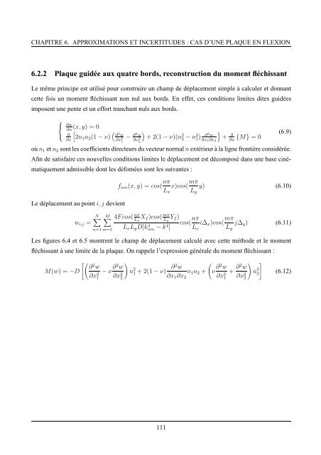
6.2.2 Plaque guidée aux quatre bords, reconstruction du moment fléchissant
Le même principe est utilisé pour construire un champ de déplacement simple à calculer et donnant
cette fois un moment fléchissant non nul aux bords. En effet, ces conditions limites dites guidées
imposent une pente et un effort tranchant nuls aux bords.
⎧
⎨
⎩
∂w
∂n
∂
∂s
(x, y) = 0
[
2n1 n 2 (1 − ν) ( ∂ 2 w
∂x 2 1
) }
− ∂2 w
∂x + 2(1 − ν)(n
2 2
2
2 − n 2 1) ∂2 w
∂x 1 ∂x 2
+
∂
{M} = 0 (6.9)
∂n
où n 1 et n 2 sont les coefficients directeurs du vecteur normal n extérieur à la ligne frontière considérée.
Afin de satisfaire ces nouvelles conditions limites le déplacement est décomposé dans une base cinématiquement
admissible dont les défomées sont les suivantes :
Le déplacement au point i, j devient
w i,j =
N∑
n=1 m=1
f nm (x, y) = cos( nπ
L x
x)cos( mπ
L y
y) (6.10)
M∑ 4Fcos( nπ
L x
X f )cos( mπ
L y
Y f )
L x L y D[knm 4 − k4 ]
cos( nπ
L x
i∆ x )cos( mπ
L y
j∆ y ) (6.11)
Les figures 6.4 et 6.5 montrent le champ de déplacement calculé avec cette méthode et le moment
fléchissant à une limite de la plaque. On rappele l’expression générale du moment fléchissant :
M(w) = −D
[( ∂ 2 w
∂x 2 1
)
− ν ∂2 w
n 2
∂x 2 1 + 2(1 − ν) ∂ 2 ( ) ]
w
n 1 n 2 + ν ∂2 w
+ ∂2 w
n 2
2
∂x 1 ∂x 2 ∂x 2 1 ∂x 2 2
2
(6.12)
111