- Page 1 and 2:
HANDBOOK OF SOLVENTS George Wypych,
- Page 3 and 4:
Preface Although the chemical indus
- Page 5 and 6:
Preface xxix contain or to have use
- Page 7 and 8:
1654 Acknowledgments 10.3 Solvent e
- Page 9 and 10:
Table of Contents Preface .........
- Page 11 and 12:
Table of contents iii 4.3 Polar sol
- Page 13 and 14:
Table of contents v 7.2.1.1 Rheolog
- Page 15 and 16:
Table of contents vii 9.4.4 Solvent
- Page 17 and 18:
Table of contents ix 12.2.2.1 Chemi
- Page 19 and 20:
Table of contents xi 14.4.3.1 Intro
- Page 21 and 22:
Table of contents xiii 14.19 Paints
- Page 23 and 24:
Table of contents xv 15.1.20 Gas ch
- Page 25 and 26:
Table of contents xvii 17.2.2 Movem
- Page 27 and 28:
Table of contents xix 18.4.7 Dry cl
- Page 29 and 30:
Table of contents xxi 20.7.1 Introd
- Page 31 and 32:
Table of contents xxiii 21.4.1.3 Pr
- Page 33 and 34:
Table of contents xxv 23.2.1.3 Sour
- Page 35 and 36:
2 Christian Reichardt aliphatic nit
- Page 37 and 38:
4 Christian Reichardt the knowledge
- Page 39 and 40:
2 Fundamental Principles Governing
- Page 41 and 42:
2.1 Solvent effects on chemical sys
- Page 43 and 44:
2.1 Solvent effects on chemical sys
- Page 45 and 46:
2.1 Solvent effects on chemical sys
- Page 47 and 48:
2.1 Solvent effects on chemical sys
- Page 49 and 50:
2.1 Solvent effects on chemical sys
- Page 51 and 52:
2.1 Solvent effects on chemical sys
- Page 53 and 54:
2.1 Solvent effects on chemical sys
- Page 55 and 56:
2.1 Solvent effects on chemical sys
- Page 57 and 58:
2.1 Solvent effects on chemical sys
- Page 59 and 60:
2.1 Solvent effects on chemical sys
- Page 61 and 62:
2.1 Solvent effects on chemical sys
- Page 63 and 64:
2.1 Solvent effects on chemical sys
- Page 65 and 66:
2.1 Solvent effects on chemical sys
- Page 67 and 68:
2.1 Solvent effects on chemical sys
- Page 69 and 70:
2.2 Molecular design of solvents 37
- Page 71 and 72:
2.2 Molecular design of solvents 39
- Page 73 and 74:
2.2 Molecular design of solvents 41
- Page 75 and 76:
2.3 Basic physical and chemical pro
- Page 77 and 78:
2.3 Basic physical and chemical pro
- Page 79 and 80:
2.3 Basic physical and chemical pro
- Page 81 and 82:
2.3 Basic physical and chemical pro
- Page 83 and 84:
2.3 Basic physical and chemical pro
- Page 85 and 86:
2.3 Basic physical and chemical pro
- Page 87 and 88:
2.3 Basic physical and chemical pro
- Page 89 and 90:
2.3 Basic physical and chemical pro
- Page 91 and 92:
2.3 Basic physical and chemical pro
- Page 93 and 94:
2.3 Basic physical and chemical pro
- Page 95 and 96:
2.3 Basic physical and chemical pro
- Page 97 and 98:
66 George Wypych Aprotic/Protic Ter
- Page 99 and 100:
68 George Wypych Biodegradability T
- Page 101 and 102:
70 George Wypych Figure 3.2.1. Sche
- Page 103 and 104:
72 George Wypych Figure 3.3.4. Simp
- Page 105 and 106:
74 George Wypych Synthetic routes a
- Page 107 and 108:
76 George Wypych Property minimum V
- Page 109 and 110:
78 George Wypych Property minimum V
- Page 111 and 112:
80 George Wypych Property minimum V
- Page 113 and 114:
82 George Wypych Property minimum V
- Page 115 and 116:
84 George Wypych Property minimum V
- Page 117 and 118:
86 George Wypych Property minimum V
- Page 119 and 120:
88 George Wypych Property minimum V
- Page 121 and 122:
90 George Wypych Property minimum V
- Page 123 and 124:
92 George Wypych Property minimum V
- Page 125 and 126:
94 George Wypych Property minimum V
- Page 127 and 128:
96 Tilman Hahn, Konrad Botzenhart,
- Page 129 and 130:
98 Tilman Hahn, Konrad Botzenhart,
- Page 131 and 132:
General Principles Governing Dissol
- Page 133 and 134:
4.1 Simple solvent characteristics
- Page 135 and 136:
4.1 Simple solvent characteristics
- Page 137 and 138:
4.1 Simple solvent characteristics
- Page 139 and 140:
4.1 Simple solvent characteristics
- Page 141 and 142:
4.1 Simple solvent characteristics
- Page 143 and 144:
4.1 Simple solvent characteristics
- Page 145 and 146:
4.1 Simple solvent characteristics
- Page 147 and 148:
4.1 Simple solvent characteristics
- Page 149 and 150:
4.1 Simple solvent characteristics
- Page 151 and 152:
4.1 Simple solvent characteristics
- Page 153 and 154:
4.1 Simple solvent characteristics
- Page 155 and 156:
4.2 Effect of system variables on s
- Page 157 and 158:
4.2 Effect of system variables on s
- Page 159 and 160:
4.2 Effect of system variables on s
- Page 161 and 162:
4.2 Effect of system variables on s
- Page 163 and 164:
4.3 Polar solvation dynamics 133 tr
- Page 165 and 166:
4.3 Polar solvation dynamics 135 Fo
- Page 167 and 168:
4.3 Polar solvation dynamics 137 at
- Page 169 and 170:
4.3 Polar solvation dynamics 139 li
- Page 171 and 172:
4.3 Polar solvation dynamics 141 Fi
- Page 173 and 174:
4.3 Polar solvation dynamics 143 Fi
- Page 175 and 176:
4.3 Polar solvation dynamics 145 ta
- Page 177 and 178:
4.4 Measurement of solvent activity
- Page 179 and 180:
4.4 Measurement of solvent activity
- Page 181 and 182:
4.4 Measurement of solvent activity
- Page 183 and 184:
4.4 Measurement of solvent activity
- Page 185 and 186:
4.4 Measurement of solvent activity
- Page 187 and 188:
4.4 Measurement of solvent activity
- Page 189 and 190:
4.4 Measurement of solvent activity
- Page 191 and 192:
4.4 Measurement of solvent activity
- Page 193 and 194:
4.4 Measurement of solvent activity
- Page 195 and 196:
4.4 Measurement of solvent activity
- Page 197 and 198:
4.4 Measurement of solvent activity
- Page 199 and 200:
4.4 Measurement of solvent activity
- Page 201 and 202:
4.4 Measurement of solvent activity
- Page 203 and 204:
4.4 Measurement of solvent activity
- Page 205 and 206:
4.4 Measurement of solvent activity
- Page 207 and 208:
4.4 Measurement of solvent activity
- Page 209 and 210:
4.4 Measurement of solvent activity
- Page 211 and 212:
4.4 Measurement of solvent activity
- Page 213 and 214:
4.4 Measurement of solvent activity
- Page 215 and 216:
4.4 Measurement of solvent activity
- Page 217 and 218:
4.4 Measurement of solvent activity
- Page 219 and 220:
4.4 Measurement of solvent activity
- Page 221 and 222:
4.4 Measurement of solvent activity
- Page 223 and 224:
4.4 Measurement of solvent activity
- Page 225 and 226:
4.4 Measurement of solvent activity
- Page 227 and 228:
4.4 Measurement of solvent activity
- Page 229 and 230:
4.4 Measurement of solvent activity
- Page 231 and 232:
4.4 Measurement of solvent activity
- Page 233 and 234:
4.4 Measurement of solvent activity
- Page 235 and 236:
4.4 Measurement of solvent activity
- Page 237 and 238:
4.4 Measurement of solvent activity
- Page 239 and 240:
4.4 Measurement of solvent activity
- Page 241 and 242:
4.4 Measurement of solvent activity
- Page 243 and 244:
4.4 Measurement of solvent activity
- Page 245 and 246:
4.4 Measurement of solvent activity
- Page 247 and 248:
4.4 Measurement of solvent activity
- Page 249 and 250:
4.4 Measurement of solvent activity
- Page 251 and 252:
4.4 Measurement of solvent activity
- Page 253 and 254:
4.4 Measurement of solvent activity
- Page 255 and 256:
4.4 Measurement of solvent activity
- Page 257 and 258:
4.4 Measurement of solvent activity
- Page 259 and 260:
4.4 Measurement of solvent activity
- Page 261 and 262:
4.4 Measurement of solvent activity
- Page 263 and 264: 4.4 Measurement of solvent activity
- Page 265 and 266: 4.4 Measurement of solvent activity
- Page 267 and 268: 4.4 Measurement of solvent activity
- Page 269 and 270: 4.4 Measurement of solvent activity
- Page 271 and 272: 4.4 Measurement of solvent activity
- Page 273 and 274: Solubility of Selected Systems and
- Page 275 and 276: 5.1 Solubility parameters 245 ln P
- Page 277 and 278: 5.1 Solubility parameters 247 Accep
- Page 279 and 280: 5.1 Solubility parameters 249 media
- Page 281 and 282: 5.1 Solubility parameters 251 Polym
- Page 283 and 284: 5.2 Prediction of solubility parame
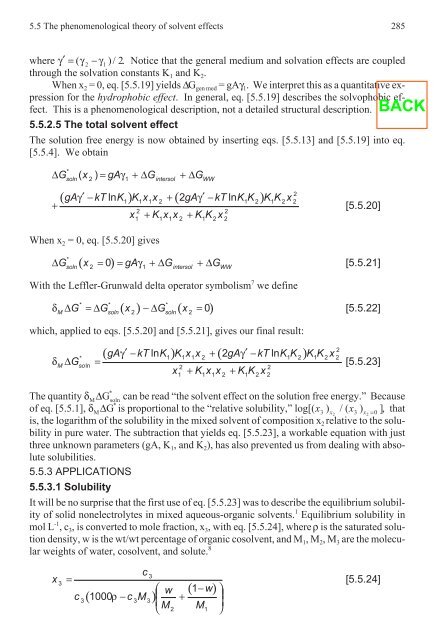
- Page 285 and 286: 5.2 Prediction of solubility parame
- Page 287 and 288: 5.2 Prediction of solubility parame
- Page 289 and 290: 5.2 Prediction of solubility parame
- Page 291 and 292: 5.3 Methods of calculation of solub
- Page 293 and 294: 5.3 Methods of calculation of solub
- Page 295 and 296: 5.3 Methods of calculation of solub
- Page 297 and 298: 5.4 Mixed solvents - polymer solubi
- Page 299 and 300: 5.4 Mixed solvents - polymer solubi
- Page 301 and 302: 5.4 Mixed solvents - polymer solubi
- Page 303 and 304: 5.4 Mixed solvents - polymer solubi
- Page 305 and 306: 5.4 Mixed solvents - polymer solubi
- Page 307 and 308: 5.4 Mixed solvents - polymer solubi
- Page 309 and 310: 5.4 Mixed solvents - polymer solubi
- Page 311 and 312: 5.5 The phenomenological theory of
- Page 313: 5.5 The phenomenological theory of
- Page 317 and 318: 5.5 The phenomenological theory of
- Page 319 and 320: 5.5 The phenomenological theory of
- Page 321 and 322: 5.5 The phenomenological theory of
- Page 323 and 324: 5.5 The phenomenological theory of
- Page 325 and 326: 5.5 The phenomenological theory of
- Page 327 and 328: 5.5 The phenomenological theory of
- Page 329 and 330: 5.5 The phenomenological theory of
- Page 331 and 332: 5.5 The phenomenological theory of
- Page 333 and 334: 5.5 The phenomenological theory of
- Page 335 and 336: 306 E. Ya. Denisyuk, V. V. Tereshat
- Page 337 and 338: 308 E. Ya. Denisyuk, V. V. Tereshat
- Page 339 and 340: 310 E. Ya. Denisyuk, V. V. Tereshat
- Page 341 and 342: 312 E. Ya. Denisyuk, V. V. Tereshat
- Page 343 and 344: 314 E. Ya. Denisyuk, V. V. Tereshat
- Page 345 and 346: 316 E. Ya. Denisyuk, V. V. Tereshat
- Page 347 and 348: 318 V V Tereshatov, V Yu. Senichev,
- Page 349 and 350: 320 V V Tereshatov, V Yu. Senichev,
- Page 351 and 352: 322 V V Tereshatov, V Yu. Senichev,
- Page 353 and 354: 324 V V Tereshatov, V Yu. Senichev,
- Page 355 and 356: 326 V V Tereshatov, V Yu. Senichev,
- Page 357 and 358: 328 Vasiliy V. Tereshatov, Valery Y
- Page 359 and 360: 330 Vasiliy V. Tereshatov, Valery Y
- Page 361 and 362: 332 Vasiliy V. Tereshatov, Valery Y
- Page 363 and 364: 334 Vasiliy V. Tereshatov, Valery Y
- Page 365 and 366:
336 Vasiliy V. Tereshatov, Valery Y
- Page 367 and 368:
338 Vasiliy V. Tereshatov, Valery Y
- Page 369 and 370:
340 George Wypych where: τM the mo
- Page 371 and 372:
342 George Wypych ξ 0.55 0.5 0.45
- Page 373 and 374:
344 George Wypych Self-diffusion co
- Page 375 and 376:
346 George Wypych Temperature, K 31
- Page 377 and 378:
348 George Wypych Diffusion distanc
- Page 379 and 380:
350 George Wypych • evaporation-i
- Page 381 and 382:
352 George Wypych Water volume frac
- Page 383 and 384:
354 George Wypych Diffusion coeffic
- Page 385 and 386:
356 Semyon Levitsky, Zinoviy Shulma
- Page 387 and 388:
358 Semyon Levitsky, Zinoviy Shulma
- Page 389 and 390:
360 Semyon Levitsky, Zinoviy Shulma
- Page 391 and 392:
362 Semyon Levitsky, Zinoviy Shulma
- Page 393 and 394:
364 Semyon Levitsky, Zinoviy Shulma
- Page 395 and 396:
366 Semyon Levitsky, Zinoviy Shulma
- Page 397 and 398:
368 Semyon Levitsky, Zinoviy Shulma
- Page 399 and 400:
370 Semyon Levitsky, Zinoviy Shulma
- Page 401 and 402:
372 Semyon Levitsky, Zinoviy Shulma
- Page 403 and 404:
374 Semyon Levitsky, Zinoviy Shulma
- Page 405 and 406:
376 Semyon Levitsky, Zinoviy Shulma
- Page 407 and 408:
378 Semyon Levitsky, Zinoviy Shulma
- Page 409 and 410:
380 Semyon Levitsky, Zinoviy Shulma
- Page 411 and 412:
382 Semyon Levitsky, Zinoviy Shulma
- Page 413 and 414:
384 Semyon Levitsky, Zinoviy Shulma
- Page 415 and 416:
386 Seung Su Kim, Jae Chun Hyun 7.3
- Page 417 and 418:
388 Seung Su Kim, Jae Chun Hyun rat
- Page 419 and 420:
390 Seung Su Kim, Jae Chun Hyun The
- Page 421 and 422:
392 Seung Su Kim, Jae Chun Hyun whe
- Page 423 and 424:
394 Seung Su Kim, Jae Chun Hyun beg
- Page 425 and 426:
396 Seung Su Kim, Jae Chun Hyun 7.3
- Page 427 and 428:
398 Seung Su Kim, Jae Chun Hyun Fig
- Page 429 and 430:
400 Seung Su Kim, Jae Chun Hyun Fig
- Page 431 and 432:
402 Seung Su Kim, Jae Chun Hyun Fig
- Page 433 and 434:
404 Seung Su Kim, Jae Chun Hyun sol
- Page 435 and 436:
406 Seung Su Kim, Jae Chun Hyun Tab
- Page 437 and 438:
408 Seung Su Kim, Jae Chun Hyun and
- Page 439 and 440:
410 Seung Su Kim, Jae Chun Hyun to
- Page 441 and 442:
412 Seung Su Kim, Jae Chun Hyun The
- Page 443 and 444:
414 Seung Su Kim, Jae Chun Hyun cau
- Page 445 and 446:
416 Seung Su Kim, Jae Chun Hyun Nu
- Page 447 and 448:
Interactions in Solvents and Soluti
- Page 449 and 450:
8.2 Basic simplifications of quantu
- Page 451 and 452:
8.2 Basic simplifications of quantu
- Page 453 and 454:
8.4 Two-body interaction energy 425
- Page 455 and 456:
8.4 Two-body interaction energy 427
- Page 457 and 458:
8.4 Two-body interaction energy 429
- Page 459 and 460:
8.4 Two-body interaction energy 431
- Page 461 and 462:
8.4 Two-body interaction energy 433
- Page 463 and 464:
8.4 Two-body interaction energy 435
- Page 465 and 466:
8.4 Two-body interaction energy 437
- Page 467 and 468:
8.4 Two-body interaction energy 439
- Page 469 and 470:
8.4 Two-body interaction energy 441
- Page 471 and 472:
8.4 Two-body interaction energy 443
- Page 473 and 474:
8.4 Two-body interaction energy 445
- Page 475 and 476:
8.4 Two-body interaction energy 447
- Page 477 and 478:
8.4 Two-body interaction energy 449
- Page 479 and 480:
8.5 Three- and many-body interactio
- Page 481 and 482:
8.5 Three- and many-body interactio
- Page 483 and 484:
8.5 Three- and many-body interactio
- Page 485 and 486:
8.6 The variety of interaction pote
- Page 487 and 488:
8.6 The variety of interaction pote
- Page 489 and 490:
8.7 Theoretical and computing model
- Page 491 and 492:
8.7 Theoretical and computing model
- Page 493 and 494:
8.7 Theoretical and computing model
- Page 495 and 496:
8.7 Theoretical and computing model
- Page 497 and 498:
8.7 Theoretical and computing model
- Page 499 and 500:
8.7 Theoretical and computing model
- Page 501 and 502:
8.7 Theoretical and computing model
- Page 503 and 504:
8.7 Theoretical and computing model
- Page 505 and 506:
8.7 Theoretical and computing model
- Page 507 and 508:
8.7 Theoretical and computing model
- Page 509 and 510:
8.7 Theoretical and computing model
- Page 511 and 512:
8.7 Theoretical and computing model
- Page 513 and 514:
8.7 Theoretical and computing model
- Page 515 and 516:
8.8 Practical applications of model
- Page 517 and 518:
8.8 Practical applications of model
- Page 519 and 520:
8.8 Practical applications of model
- Page 521 and 522:
8.9 Liquid surfaces 493 to study th
- Page 523 and 524:
8.9 Liquid surfaces 495 The potenti
- Page 525 and 526:
8.9 Liquid surfaces 497 out of equi
- Page 527 and 528:
8.9 Liquid surfaces 499 tions) of t
- Page 529 and 530:
8 Interactions in solvents and solu
- Page 531 and 532:
8 Interactions in solvents and solu
- Page 533 and 534:
9 Mixed Solvents Y. Y. Fialkov, V.
- Page 535 and 536:
9.2 Chemical interaction between co
- Page 537 and 538:
9.2 Chemical interaction between co
- Page 539 and 540:
9.3 Physical properties of mixed so
- Page 541 and 542:
9.3 Physical properties of mixed so
- Page 543 and 544:
9.3 Physical properties of mixed so
- Page 545 and 546:
9.3 Physical properties of mixed so
- Page 547 and 548:
9.3 Physical properties of mixed so
- Page 549 and 550:
9.3 Physical properties of mixed so
- Page 551 and 552:
9.3 Physical properties of mixed so
- Page 553 and 554:
9.3 Physical properties of mixed so
- Page 555 and 556:
9.4 Mixed solvent influence on the
- Page 557 and 558:
9.4 Mixed solvent influence on the
- Page 559 and 560:
9.4 Mixed solvent influence on the
- Page 561 and 562:
9.4 Mixed solvent influence on the
- Page 563 and 564:
9.4 Mixed solvent influence on the
- Page 565 and 566:
9.4 Mixed solvent influence on the
- Page 567 and 568:
9.4 Mixed solvent influence on the
- Page 569 and 570:
9.4 Mixed solvent influence on the
- Page 571 and 572:
9.4 Mixed solvent influence on the
- Page 573 and 574:
9.4 Mixed solvent influence on the
- Page 575 and 576:
9.4 Mixed solvent influence on the
- Page 577 and 578:
9.4 Mixed solvent influence on the
- Page 579 and 580:
9.4 Mixed solvent influence on the
- Page 581 and 582:
9.4 Mixed solvent influence on the
- Page 583 and 584:
9.4 Mixed solvent influence on the
- Page 585 and 586:
9.5 The mixed solvent effect on the
- Page 587 and 588:
9.5 The mixed solvent effect on the
- Page 589 and 590:
9.5 The mixed solvent effect on the
- Page 591 and 592:
9 Mixed solvents 563 22 Minkin V.,
- Page 593 and 594:
10 Acid-base Interactions 10.1 GENE
- Page 595 and 596:
10.1 General concept of acid-base i
- Page 597 and 598:
10.1 General concept of acid-base i
- Page 599 and 600:
10.2 Effect of polymer/solvent acid
- Page 601 and 602:
10.2 Effect of polymer/solvent acid
- Page 603 and 604:
10.2 Effect of polymer/solvent acid
- Page 605 and 606:
10.2 Effect of polymer/solvent acid
- Page 607 and 608:
10.2 Effect of polymer/solvent acid
- Page 609 and 610:
10.2 Effect of polymer/solvent acid
- Page 611 and 612:
10.3 Solvent effects based on pure
- Page 613 and 614:
10.3 Solvent effects based on pure
- Page 615 and 616:
10.3 Solvent effects based on pure
- Page 617 and 618:
10.3 Solvent effects based on pure
- Page 619 and 620:
10.3 Solvent effects based on pure
- Page 621 and 622:
10.3 Solvent effects based on pure
- Page 623 and 624:
10.3 Solvent effects based on pure
- Page 625 and 626:
10.3 Solvent effects based on pure
- Page 627 and 628:
10.3 Solvent effects based on pure
- Page 629 and 630:
10.3 Solvent effects based on pure
- Page 631 and 632:
10.3 Solvent effects based on pure
- Page 633 and 634:
10.3 Solvent effects based on pure
- Page 635 and 636:
10.3 Solvent effects based on pure
- Page 637 and 638:
10.3 Solvent effects based on pure
- Page 639 and 640:
10.3 Solvent effects based on pure
- Page 641 and 642:
10.3 Solvent effects based on pure
- Page 643 and 644:
10.3 Solvent effects based on pure
- Page 645 and 646:
10.4 Acid-base equilibria in ionic
- Page 647 and 648:
10.4 Acid-base equilibria in ionic
- Page 649 and 650:
10.4 Acid-base equilibria in ionic
- Page 651 and 652:
10.4 Acid-base equilibria in ionic
- Page 653 and 654:
10.4 Acid-base equilibria in ionic
- Page 655 and 656:
10.4 Acid-base equilibria in ionic
- Page 657 and 658:
10.4 Acid-base equilibria in ionic
- Page 659 and 660:
10.4 Acid-base equilibria in ionic
- Page 661 and 662:
10.4 Acid-base equilibria in ionic
- Page 663 and 664:
10.4 Acid-base equilibria in ionic
- Page 665 and 666:
10.4 Acid-base equilibria in ionic
- Page 667 and 668:
11 Electronic and Electrical Effect
- Page 669 and 670:
11.1 Theoretical treatment of solve
- Page 671 and 672:
11.1 Theoretical treatment of solve
- Page 673 and 674:
11.1 Theoretical treatment of solve
- Page 675 and 676:
11.1 Theoretical treatment of solve
- Page 677 and 678:
11.1 Theoretical treatment of solve
- Page 679 and 680:
11.1 Theoretical treatment of solve
- Page 681 and 682:
11.1 Theoretical treatment of solve
- Page 683 and 684:
11.1 Theoretical treatment of solve
- Page 685 and 686:
11.1 Theoretical treatment of solve
- Page 687 and 688:
11.1 Theoretical treatment of solve
- Page 689 and 690:
11.1 Theoretical treatment of solve
- Page 691 and 692:
11.1 Theoretical treatment of solve
- Page 693 and 694:
11.1 Theoretical treatment of solve
- Page 695 and 696:
11.1 Theoretical treatment of solve
- Page 697 and 698:
11.1 Theoretical treatment of solve
- Page 699 and 700:
11.1 Theoretical treatment of solve
- Page 701 and 702:
11.1 Theoretical treatment of solve
- Page 703 and 704:
11.1 Theoretical treatment of solve
- Page 705 and 706:
11.1 Theoretical treatment of solve
- Page 707 and 708:
11.1 Theoretical treatment of solve
- Page 709 and 710:
11.2 Dielectric solvent effects 681
- Page 711 and 712:
12 Other Properties of Solvents, So
- Page 713 and 714:
12.1 Rheological properties, aggreg
- Page 715 and 716:
12.1 Rheological properties, aggreg
- Page 717 and 718:
12.1 Rheological properties, aggreg
- Page 719 and 720:
12.1 Rheological properties, aggreg
- Page 721 and 722:
12.1 Rheological properties, aggreg
- Page 723 and 724:
12.1 Rheological properties, aggreg
- Page 725 and 726:
12.1 Rheological properties, aggreg
- Page 727 and 728:
12.1 Rheological properties, aggreg
- Page 729 and 730:
12.1 Rheological properties, aggreg
- Page 731 and 732:
12.1 Rheological properties, aggreg
- Page 733 and 734:
12.1 Rheological properties, aggreg
- Page 735 and 736:
12.2 Chain conformations of polysac
- Page 737 and 738:
12.2 Chain conformations of polysac
- Page 739 and 740:
12.2 Chain conformations of polysac
- Page 741 and 742:
12.2 Chain conformations of polysac
- Page 743 and 744:
12.2 Chain conformations of polysac
- Page 745 and 746:
12.2 Chain conformations of polysac
- Page 747 and 748:
12.2 Chain conformations of polysac
- Page 749 and 750:
12.2 Chain conformations of polysac
- Page 751 and 752:
12.2 Chain conformations of polysac
- Page 753 and 754:
12.2 Chain conformations of polysac
- Page 755 and 756:
12.2 Chain conformations of polysac
- Page 757 and 758:
12.2 Chain conformations of polysac
- Page 759 and 760:
12.2 Chain conformations of polysac
- Page 761 and 762:
12.2 Chain conformations of polysac
- Page 763 and 764:
12.2 Chain conformations of polysac
- Page 765 and 766:
738 Roland Schmid Figure 13.1.1. Re
- Page 767 and 768:
740 Roland Schmid HB interactions,
- Page 769 and 770:
742 Roland Schmid AN = -133.8 - 0.0
- Page 771 and 772:
744 Roland Schmid ated by the macro
- Page 773 and 774:
746 Roland Schmid turns out, polar
- Page 775 and 776:
748 Roland Schmid Packing density
- Page 777 and 778:
750 Roland Schmid tween calculated
- Page 779 and 780:
752 Roland Schmid over the solute-s
- Page 781 and 782:
754 Roland Schmid of the empirical
- Page 783 and 784:
756 Roland Schmid From X-ray and ne
- Page 785 and 786:
758 Roland Schmid Table 13.1.5. Sol
- Page 787 and 788:
760 Roland Schmid ΔG = ΔG + ΔG [
- Page 789 and 790:
762 Roland Schmid very recent paper
- Page 791 and 792:
764 Roland Schmid Solvent ΔvH/RT
- Page 793 and 794:
766 Roland Schmid E r = E i + E s [
- Page 795 and 796:
768 Roland Schmid from the explicit
- Page 797 and 798:
770 Roland Schmid sequently, there
- Page 799 and 800:
772 Roland Schmid simulations. 188-
- Page 801 and 802:
774 Roland Schmid 23 N. A. Lewis, Y
- Page 803 and 804:
776 Roland Schmid 132 R. R. Dogonad
- Page 805 and 806:
778 Michelle L. Coote and Thomas P.
- Page 807 and 808:
780 Michelle L. Coote and Thomas P.
- Page 809 and 810:
782 Michelle L. Coote and Thomas P.
- Page 811 and 812:
784 Michelle L. Coote and Thomas P.
- Page 813 and 814:
786 Michelle L. Coote and Thomas P.
- Page 815 and 816:
788 Michelle L. Coote and Thomas P.
- Page 817 and 818:
790 Michelle L. Coote and Thomas P.
- Page 819 and 820:
792 Michelle L. Coote and Thomas P.
- Page 821 and 822:
794 Michelle L. Coote and Thomas P.
- Page 823 and 824:
796 Michelle L. Coote and Thomas P.
- Page 825 and 826:
798 Maw-Ling Wang 13.3 EFFECTS OF O
- Page 827 and 828:
800 Maw-Ling Wang [13.3.2] Inverse
- Page 829 and 830:
802 Maw-Ling Wang Both cation and a
- Page 831 and 832:
804 Maw-Ling Wang Table 13.3.2. Eff
- Page 833 and 834:
806 Maw-Ling Wang Table 13.3.3. Ext
- Page 835 and 836:
808 Maw-Ling Wang Table 13.3.5. Eff
- Page 837 and 838:
810 Maw-Ling Wang reacts with pheno
- Page 839 and 840:
812 Maw-Ling Wang Figure 13.3.3. Ef
- Page 841 and 842:
814 Maw-Ling Wang the organic solve
- Page 843 and 844:
816 Maw-Ling Wang crease. Therefore
- Page 845 and 846:
818 Maw-Ling Wang (F) Polymerizatio
- Page 847 and 848:
820 Maw-Ling Wang Table 13.3.16. Sy
- Page 849 and 850:
822 Maw-Ling Wang 13.3.1.4 Effect o
- Page 851 and 852:
824 Maw-Ling Wang Table 13.3.19 Eff
- Page 853 and 854:
826 Maw-Ling Wang quaternary salt c
- Page 855 and 856:
828 Maw-Ling Wang Table 13.3.24. Ef
- Page 857 and 858:
830 Maw-Ling Wang Solvent Dielectri
- Page 859 and 860:
832 Maw-Ling Wang ied. 82,83,97,101
- Page 861 and 862:
834 Maw-Ling Wang substitution, suc
- Page 863 and 864:
836 Maw-Ling Wang (2) the ion excha
- Page 865 and 866:
838 Maw-Ling Wang REFERENCES 1 A. A
- Page 867 and 868:
840 Maw-Ling Wang 101 D. C. Sherrin
- Page 869 and 870:
842 Norio Tsubokawa [13.4.2] PAI is
- Page 871 and 872:
844 Norio Tsubokawa Table 13.4.2. I
- Page 873 and 874:
846 Norio Tsubokawa more easily tha
- Page 875 and 876:
848 George Wypych methyl amyl keton
- Page 877 and 878:
850 George Wypych Peel strength, N/
- Page 879 and 880:
852 George Wypych 8 P Enenkel, H Ba
- Page 881 and 882:
854 George Wypych Table 14.2.2. Tot
- Page 883 and 884:
856 M Matsumoto, S Isken, JAMdeBont
- Page 885 and 886:
858 M Matsumoto, S Isken, JAMdeBont
- Page 887 and 888:
860 M Matsumoto, S Isken, JAMdeBont
- Page 889 and 890:
862 M Matsumoto, S Isken, JAMdeBont
- Page 891 and 892:
864 M Matsumoto, S Isken, JAMdeBont
- Page 893 and 894:
866 Tilman Hahn, Konrad Botzenhart
- Page 895 and 896:
868 Tilman Hahn, Konrad Botzenhart
- Page 897 and 898:
870 Tilman Hahn, Konrad Botzenhart
- Page 899 and 900:
872 Tsuneo Yamane 14.4.3 CHOICE OF
- Page 901 and 902:
874 Tsuneo Yamane Very trace amount
- Page 903 and 904:
876 Tsuneo Yamane It has been shown
- Page 905 and 906:
878 Tsuneo Yamane [ ( kcat Km) ( kc
- Page 907 and 908:
880 George Wypych 11 A. Zaks, in En
- Page 909 and 910:
882 George Wypych rected towards im
- Page 911 and 912:
884 Kaspar D. Hasenclever than 55°
- Page 913 and 914:
886 Kaspar D. Hasenclever The same
- Page 915 and 916:
888 Kaspar D. Hasenclever Figure 14
- Page 917 and 918:
890 Kaspar D. Hasenclever Computer
- Page 919 and 920:
892 Kaspar D. Hasenclever • Solve
- Page 921 and 922:
894 Martin Hanek, Norbert Löw, And
- Page 923 and 924:
896 Martin Hanek, Norbert Löw, And
- Page 925 and 926:
898 Martin Hanek, Norbert Löw, And
- Page 927 and 928:
900 Martin Hanek, Norbert Löw, And
- Page 929 and 930:
902 Martin Hanek, Norbert Löw, And
- Page 931 and 932:
904 Martin Hanek, Norbert Löw, And
- Page 933 and 934:
906 Martin Hanek, Norbert Löw, And
- Page 935 and 936:
908 Martin Hanek, Norbert Löw, And
- Page 937 and 938:
910 Martin Hanek, Norbert Löw, And
- Page 939 and 940:
912 Martin Hanek, Norbert Löw, And
- Page 941 and 942:
914 Martin Hanek, Norbert Löw, And
- Page 943 and 944:
916 Martin Hanek, Norbert Löw, And
- Page 945 and 946:
918 Martin Hanek, Norbert Löw, And
- Page 947 and 948:
920 George Wypych 20 N. L�w, EPP
- Page 949 and 950:
922 George Wypych Table 14.9.2. Rep
- Page 951 and 952:
924 Phillip J. Wakelyn, Peter J. Wa
- Page 953 and 954:
926 Phillip J. Wakelyn, Peter J. Wa
- Page 955 and 956:
928 Phillip J. Wakelyn, Peter J. Wa
- Page 957 and 958:
930 Phillip J. Wakelyn, Peter J. Wa
- Page 959 and 960:
932 Phillip J. Wakelyn, Peter J. Wa
- Page 961 and 962:
934 Phillip J. Wakelyn, Peter J. Wa
- Page 963 and 964:
936 Phillip J. Wakelyn, Peter J. Wa
- Page 965 and 966:
938 Phillip J. Wakelyn, Peter J. Wa
- Page 967 and 968:
940 Phillip J. Wakelyn, Peter J. Wa
- Page 969 and 970:
942 Phillip J. Wakelyn, Peter J. Wa
- Page 971 and 972:
944 Phillip J. Wakelyn, Peter J. Wa
- Page 973 and 974:
946 Phillip J. Wakelyn, Peter J. Wa
- Page 975 and 976:
948 Phillip J. Wakelyn, Peter J. Wa
- Page 977 and 978:
950 George Wypych 14.11 GROUND TRAN
- Page 979 and 980:
952 George Wypych Figure 14.13.1. S
- Page 981 and 982:
954 Tilman Hahn, Konrad Botzenhart,
- Page 983 and 984:
956 George Wypych more to show that
- Page 985 and 986:
958 George Wypych Table 14.16.1. Re
- Page 987 and 988:
960 George Wypych Table 14.17.1. Re
- Page 989 and 990:
962 George Wypych Table 14.18.2. Re
- Page 991 and 992:
964 Tilman Hahn, Konrad Botzenhart,
- Page 993 and 994:
966 Tilman Hahn, Konrad Botzenhart,
- Page 995 and 996:
968 Tilman Hahn, Konrad Botzenhart,
- Page 997 and 998:
970 David Randall 14.19.2.2 Water b
- Page 999 and 1000:
972 David Randall Hydrophobic subst
- Page 1001 and 1002:
974 David Randall 50-60% glutaric,
- Page 1003 and 1004:
976 George Wypych Figure 14.20.1. D
- Page 1005 and 1006:
978 Michel Bauer, Christine Barthé
- Page 1007 and 1008:
980 Michel Bauer, Christine Barthé
- Page 1009 and 1010:
982 Michel Bauer, Christine Barthé
- Page 1011 and 1012:
984 Michel Bauer, Christine Barthé
- Page 1013 and 1014:
986 Michel Bauer, Christine Barthé
- Page 1015 and 1016:
988 Michel Bauer, Christine Barthé
- Page 1017 and 1018:
990 Michel Bauer, Christine Barthé
- Page 1019 and 1020:
992 Michel Bauer, Christine Barthé
- Page 1021 and 1022:
994 Michel Bauer, Christine Barthé
- Page 1023 and 1024:
996 Michel Bauer, Christine Barthé
- Page 1025 and 1026:
998 An Li This discussion is intend
- Page 1027 and 1028:
1000 An Li Trade Name Cosolvent vol
- Page 1029 and 1030:
1002 An Li Figure 14.21.2.1. Effect
- Page 1031 and 1032:
1004 An Li partial derivative ∂(l
- Page 1033 and 1034:
1006 An Li Equation [14.21.2.8] can
- Page 1035 and 1036:
1008 An Li Figure 14.21.2.2a. Devia
- Page 1037 and 1038:
1010 An Li Figure 14.21.2.2c. Devia
- Page 1039 and 1040:
1012 An Li f 0.1 0.2 0.4 0.6 0.8 0.
- Page 1041 and 1042:
1014 An Li estimated from the log K
- Page 1043 and 1044:
1016 George Wypych 72 K. Brololm, a
- Page 1045 and 1046:
1018 George Wypych Figure 14.22.2.
- Page 1047 and 1048:
1020 George Wypych New technology i
- Page 1049 and 1050:
1022 George Wypych Table 14.23.1. R
- Page 1051 and 1052:
1024 George Wypych Table 14.24.2. R
- Page 1053 and 1054:
1026 Mohamed Serageldin, Dave Reeve
- Page 1055 and 1056:
1028 Mohamed Serageldin, Dave Reeve
- Page 1057 and 1058:
1030 Mohamed Serageldin, Dave Reeve
- Page 1059 and 1060:
1032 Mohamed Serageldin, Dave Reeve
- Page 1061 and 1062:
1034 Mohamed Serageldin, Dave Reeve
- Page 1063 and 1064:
1036 Mohamed Serageldin, Dave Reeve
- Page 1065 and 1066:
1038 Mohamed Serageldin, Dave Reeve
- Page 1067 and 1068:
1040 George Wypych Table 14.27.2. R
- Page 1069 and 1070:
1042 George Wypych Table 14.28.2. R
- Page 1071 and 1072:
1044 George Wypych Table 14.31.1. R
- Page 1073 and 1074:
1046 George Wypych Table 14.32.1. R
- Page 1075 and 1076:
1048 George Wypych Table 14.32.3. R
- Page 1077 and 1078:
1050 George Wypych Table 14.32.5. T
- Page 1079 and 1080:
1052 George Wypych The traditional
- Page 1081 and 1082:
1054 George Wypych The acidity of b
- Page 1083 and 1084:
1056 George Wypych except water whi
- Page 1085 and 1086:
1058 George Wypych solution is 2.73
- Page 1087 and 1088:
1060 George Wypych presence of igni
- Page 1089 and 1090:
1062 George Wypych method of determ
- Page 1091 and 1092:
1064 George Wypych used. A thermal
- Page 1093 and 1094:
1066 George Wypych 15.1.26 REFRACTI
- Page 1095 and 1096:
1068 George Wypych Table 15.1.1. Ty
- Page 1097 and 1098:
1070 George Wypych Wexcluded solven
- Page 1099 and 1100:
1072 George Wypych 25 ASTM D 2108-9
- Page 1101 and 1102:
1074 George Wypych 68 ASTM D 3844-9
- Page 1103 and 1104:
1076 George Wypych BS 506-2.84. Met
- Page 1105 and 1106:
1078 Myrto Petreas 15.2 SPECIAL MET
- Page 1107 and 1108:
1080 Myrto Petreas In short, biolog
- Page 1109 and 1110:
1082 Myrto Petreas cients of some i
- Page 1111 and 1112:
1084 Myrto Petreas lection at the a
- Page 1113 and 1114:
1086 Myrto Petreas and legal reperc
- Page 1115 and 1116:
1088 Myrto Petreas • The solvent
- Page 1117 and 1118:
1090 Myrto Petreas of time after ex
- Page 1119 and 1120:
1092 Myrto Petreas even after log-l
- Page 1121 and 1122:
1094 Myrto Petreas 26 M Petreas, J
- Page 1123 and 1124:
1096 James L. Botsford In Europe ma
- Page 1125 and 1126:
1098 James L. Botsford Figure 15.2.
- Page 1127 and 1128:
1100 James L. Botsford cussed. Neit
- Page 1129 and 1130:
1102 James L. Botsford n Ave. Var.
- Page 1131 and 1132:
1104 James L. Botsford (Calleja et
- Page 1133 and 1134:
1106 James L. Botsford Table 15.2.2
- Page 1135 and 1136:
1108 James L. Botsford the test is
- Page 1137 and 1138:
1110 James L. Botsford Table 15.2.2
- Page 1139 and 1140:
1112 James L. Botsford Geiger, D. L
- Page 1141 and 1142:
1114 Christine Barthélémy, Michel
- Page 1143 and 1144:
1116 Christine Barthélémy, Michel
- Page 1145 and 1146:
1118 Christine Barthélémy, Michel
- Page 1147 and 1148:
1120 Christine Barthélémy, Michel
- Page 1149 and 1150:
1122 Christine Barthélémy, Michel
- Page 1151 and 1152:
1124 Christine Barthélémy, Michel
- Page 1153 and 1154:
1126 George Wypych n-heptane molecu
- Page 1155 and 1156:
1128 George Wypych MEK P PA Fat-fre
- Page 1157 and 1158:
1130 Michel Bauer, Christine Barth
- Page 1159 and 1160:
1132 Michel Bauer, Christine Barth
- Page 1161 and 1162:
1134 Michel Bauer, Christine Barth
- Page 1163 and 1164:
1136 Michel Bauer, Christine Barth
- Page 1165 and 1166:
1138 Michel Bauer, Christine Barth
- Page 1167 and 1168:
1140 Michel Bauer, Christine Barth
- Page 1169 and 1170:
1142 Michel Bauer, Christine Barth
- Page 1171 and 1172:
1144 Michel Bauer, Christine Barth
- Page 1173 and 1174:
1146 Michel Bauer, Christine Barth
- Page 1175 and 1176:
17 Environmental Impact of Solvents
- Page 1177 and 1178:
17.1 The environmental fate and mov
- Page 1179 and 1180:
17.1 The environmental fate and mov
- Page 1181 and 1182:
17.1 The environmental fate and mov
- Page 1183 and 1184:
17.1 The environmental fate and mov
- Page 1185 and 1186:
17.1 The environmental fate and mov
- Page 1187 and 1188:
17.1 The environmental fate and mov
- Page 1189 and 1190:
17.2 Fate-based management 1163 dat
- Page 1191 and 1192:
17.2 Fate-based management 1165 bre
- Page 1193 and 1194:
17.2 Fate-based management 1167 gra
- Page 1195 and 1196:
17.3 Environmental fate of glycol e
- Page 1197 and 1198:
17.3 Environmental fate of glycol e
- Page 1199 and 1200:
17.3 Environmental fate of glycol e
- Page 1201 and 1202:
17.3 Environmental fate of glycol e
- Page 1203 and 1204:
17.3 Environmental fate of glycol e
- Page 1205 and 1206:
17.3 Environmental fate of glycol e
- Page 1207 and 1208:
17.3 Environmental fate of glycol e
- Page 1209 and 1210:
17.3 Environmental fate of glycol e
- Page 1211 and 1212:
17.3 Environmental fate of glycol e
- Page 1213 and 1214:
17.3 Environmental fate of glycol e
- Page 1215 and 1216:
17.4 Organic solvent impacts on tro
- Page 1217 and 1218:
17.4 Organic solvent impacts on tro
- Page 1219 and 1220:
17.4 Organic solvent impacts on tro
- Page 1221 and 1222:
17.4 Organic solvent impacts on tro
- Page 1223 and 1224:
17.4 Organic solvent impacts on tro
- Page 1225 and 1226:
17.4 Organic solvent impacts on tro
- Page 1227 and 1228:
18 Concentration of Solvents in Var
- Page 1229 and 1230:
18.1 Measurement and estimation of
- Page 1231 and 1232:
18.1 Measurement and estimation of
- Page 1233 and 1234:
18.1 Measurement and estimation of
- Page 1235 and 1236:
18.1 Measurement and estimation of
- Page 1237 and 1238:
18.1 Measurement and estimation of
- Page 1239 and 1240:
18.1 Measurement and estimation of
- Page 1241 and 1242:
18.1 Measurement and estimation of
- Page 1243 and 1244:
18.1 Measurement and estimation of
- Page 1245 and 1246:
18.1 Measurement and estimation of
- Page 1247 and 1248:
18.1 Measurement and estimation of
- Page 1249 and 1250:
18.1 Measurement and estimation of
- Page 1251 and 1252:
18.1 Measurement and estimation of
- Page 1253 and 1254:
18.2 Prediction of organic solvents
- Page 1255 and 1256:
18.2 Prediction of organic solvents
- Page 1257 and 1258:
18.2 Prediction of organic solvents
- Page 1259 and 1260:
18.2 Prediction of organic solvents
- Page 1261 and 1262:
18.3 Indoor air pollution by solven
- Page 1263 and 1264:
18.3 Indoor air pollution by solven
- Page 1265 and 1266:
18.3 Indoor air pollution by solven
- Page 1267 and 1268:
18.3 Indoor air pollution by solven
- Page 1269 and 1270:
18.3 Indoor air pollution by solven
- Page 1271 and 1272:
18.3 Indoor air pollution by solven
- Page 1273 and 1274:
18.3 Indoor air pollution by solven
- Page 1275 and 1276:
18.3 Indoor air pollution by solven
- Page 1277 and 1278:
18.4 Solvent uses with exposure ris
- Page 1279 and 1280:
18.4 Solvent uses with exposure ris
- Page 1281 and 1282:
18.4 Solvent uses with exposure ris
- Page 1283 and 1284:
18.4 Solvent uses with exposure ris
- Page 1285 and 1286:
18.4 Solvent uses with exposure ris
- Page 1287 and 1288:
18.4 Solvent uses with exposure ris
- Page 1289 and 1290:
18.4 Solvent uses with exposure ris
- Page 1291 and 1292:
18.4 Solvent uses with exposure ris
- Page 1293 and 1294:
1268 Carlos M. Nu�ez ter or habit
- Page 1295 and 1296:
1270 Carlos M. Nu�ez CAS No. Chem
- Page 1297 and 1298:
1272 Carlos M. Nu�ez CAS No. Chem
- Page 1299 and 1300:
1274 Carlos M. Nu�ez CAS No. Chem
- Page 1301 and 1302:
1276 Carlos M. Nu�ez CAS No. Chem
- Page 1303 and 1304:
1278 Carlos M. Nu�ez CAS No. Chem
- Page 1305 and 1306:
1280 Carlos M. Nu�ez CAS No. Chem
- Page 1307 and 1308:
1282 Carlos M. Nu�ez tronic circu
- Page 1309 and 1310:
1284 Carlos M. Nu�ez EPA Region 6
- Page 1311 and 1312:
1286 Carlos M. Nu�ez i.e., entire
- Page 1313 and 1314:
1288 Carlos M. Nu�ez Table 19.6.
- Page 1315 and 1316:
1290 Carlos M. Nu�ez Schedule Sou
- Page 1317 and 1318:
1292 Carlos M. Nu�ez The CAA prov
- Page 1319 and 1320:
1294 Carlos M. Nu�ez CWA to estab
- Page 1321 and 1322:
1296 Carlos M. Nu�ez amended to i
- Page 1323 and 1324:
1298 Carlos M. Nu�ez Figure 19.5.
- Page 1325 and 1326:
1300 Carlos M. Nu�ez environmenta
- Page 1327 and 1328:
1302 Carlos M. Nu�ez For comparis
- Page 1329 and 1330:
1304 Carlos M. Nu�ez tives. Four
- Page 1331 and 1332:
1306 Carlos M. Nu�ez • Program
- Page 1333 and 1334:
1308 Carlos M. Nu�ez 31 Federal R
- Page 1335 and 1336:
1310 Carlos M. Nu�ez HSWA Hazardo
- Page 1337 and 1338:
1312 Tilman Hahn, Konrad Botzenhart
- Page 1339 and 1340:
20 Toxic Effects of Solvent Exposur
- Page 1341 and 1342:
20.1 Toxicokinetics, toxicodynamics
- Page 1343 and 1344:
20.1 Toxicokinetics, toxicodynamics
- Page 1345 and 1346:
20.1 Toxicokinetics, toxicodynamics
- Page 1347 and 1348:
20.1 Toxicokinetics, toxicodynamics
- Page 1349 and 1350:
20.1 Toxicokinetics, toxicodynamics
- Page 1351 and 1352:
20.2 Cognitive and psychosocial out
- Page 1353 and 1354:
20.2 Cognitive and psychosocial out
- Page 1355 and 1356:
20.2 Cognitive and psychosocial out
- Page 1357 and 1358:
20.3 Pregnancy outcome following so
- Page 1359 and 1360:
20.3 Pregnancy outcome following so
- Page 1361 and 1362:
20.3 Pregnancy outcome following so
- Page 1363 and 1364:
20.3 Pregnancy outcome following so
- Page 1365 and 1366:
20.3 Pregnancy outcome following so
- Page 1367 and 1368:
20.3 Pregnancy outcome following so
- Page 1369 and 1370:
20.3 Pregnancy outcome following so
- Page 1371 and 1372:
20.3 Pregnancy outcome following so
- Page 1373 and 1374:
20.3 Pregnancy outcome following so
- Page 1375 and 1376:
20.3 Pregnancy outcome following so
- Page 1377 and 1378:
20.3 Pregnancy outcome following so
- Page 1379 and 1380:
20.4 Industrial solvents and kidney
- Page 1381 and 1382:
20.4 Industrial solvents and kidney
- Page 1383 and 1384:
20.4 Industrial solvents and kidney
- Page 1385 and 1386:
20.4 Industrial solvents and kidney
- Page 1387 and 1388:
20.5 Lymphohematopoietic study of w
- Page 1389 and 1390:
20.5 Lymphohematopoietic study of w
- Page 1391 and 1392:
20.5 Lymphohematopoietic study of w
- Page 1393 and 1394:
20.5 Lymphohematopoietic study of w
- Page 1395 and 1396:
20.5 Lymphohematopoietic study of w
- Page 1397 and 1398:
20.5 Lymphohematopoietic study of w
- Page 1399 and 1400:
20.6 Chromosomal aberrations 1375 2
- Page 1401 and 1402:
20.6 Chromosomal aberrations 1377 p
- Page 1403 and 1404:
20.7 Hepatotoxicity 1379 8 Mitelman
- Page 1405 and 1406:
20.7 Hepatotoxicity 1381 to convert
- Page 1407 and 1408:
20.7 Hepatotoxicity 1383 Table 20.7
- Page 1409 and 1410:
20.7 Hepatotoxicity 1385 toxicity o
- Page 1411 and 1412:
20.7 Hepatotoxicity 1387 early pote
- Page 1413 and 1414:
20.7 Hepatotoxicity 1389 vents. It
- Page 1415 and 1416:
20.7 Hepatotoxicity 1391 19 Slater
- Page 1417 and 1418:
20.8 Solvents and the liver 1393 20
- Page 1419 and 1420:
20.8 Solvents and the liver 1395 Cu
- Page 1421 and 1422:
20.8 Solvents and the liver 1397 th
- Page 1423 and 1424:
20.8 Solvents and the liver 1399 cu
- Page 1425 and 1426:
20.8 Solvents and the liver 1401 20
- Page 1427 and 1428:
20.8 Solvents and the liver 1403 65
- Page 1429 and 1430:
20.9 Toxicity of environmental solv
- Page 1431 and 1432:
20.9 Toxicity of environmental solv
- Page 1433 and 1434:
20.9 Toxicity of environmental solv
- Page 1435 and 1436:
20.9 Toxicity of environmental solv
- Page 1437 and 1438:
20.9 Toxicity of environmental solv
- Page 1439 and 1440:
20.9 Toxicity of environmental solv
- Page 1441 and 1442:
20.9 Toxicity of environmental solv
- Page 1443 and 1444:
21 Substitution of Solvents by Safe
- Page 1445 and 1446:
21.1 Supercritical solvents 1421 So
- Page 1447 and 1448:
21.1 Supercritical solvents 1423 Fi
- Page 1449 and 1450:
21.1 Supercritical solvents 1425 Fi
- Page 1451 and 1452:
21.1 Supercritical solvents 1427 Fi
- Page 1453 and 1454:
21.1 Supercritical solvents 1429 K
- Page 1455 and 1456:
21.1 Supercritical solvents 1431 ai
- Page 1457 and 1458:
21.1 Supercritical solvents 1433 Th
- Page 1459 and 1460:
21.1 Supercritical solvents 1435 wh
- Page 1461 and 1462:
21.1 Supercritical solvents 1437 *
- Page 1463 and 1464:
21.1 Supercritical solvents 1439 In
- Page 1465 and 1466:
21.1 Supercritical solvents 1441 21
- Page 1467 and 1468:
21.1 Supercritical solvents 1443 Ta
- Page 1469 and 1470:
21.1 Supercritical solvents 1445 Re
- Page 1471 and 1472:
21.1 Supercritical solvents 1447 Re
- Page 1473 and 1474:
21.1 Supercritical solvents 1449 ta
- Page 1475 and 1476:
21.1 Supercritical solvents 1451 21
- Page 1477 and 1478:
21.1 Supercritical solvents 1453 Fi
- Page 1479 and 1480:
21.1 Supercritical solvents 1455 Fi
- Page 1481 and 1482:
21.1 Supercritical solvents 1457 13
- Page 1483 and 1484:
21.2 Ionic liquids 1459 85 M. Polia
- Page 1485 and 1486:
21.2 Ionic liquids 1461 be used. Th
- Page 1487 and 1488:
21.2 Ionic liquids 1463 Figure 21.2
- Page 1489 and 1490:
21.2 Ionic liquids 1465 Table 21.2.
- Page 1491 and 1492:
21.2 Ionic liquids 1467 been utiliz
- Page 1493 and 1494:
21.2 Ionic liquids 1469 One specifi
- Page 1495 and 1496:
21.2 Ionic liquids 1471 lustrates t
- Page 1497 and 1498:
21.2 Ionic liquids 1473 these alloy
- Page 1499 and 1500:
21.2 Ionic liquids 1475 ( ) ln = K
- Page 1501 and 1502:
21.2 Ionic liquids 1477 According t
- Page 1503 and 1504:
21.2 Ionic liquids 1479 Acidic melt
- Page 1505 and 1506:
21.2 Ionic liquids 1481 21 C.L. Hus
- Page 1507 and 1508:
21.2 Ionic liquids 1483 110 G.P. Li
- Page 1509 and 1510:
21.3 Oxide solubilities in ionic me
- Page 1511 and 1512:
21.3 Oxide solubilities in ionic me
- Page 1513 and 1514:
21.3 Oxide solubilities in ionic me
- Page 1515 and 1516:
21.3 Oxide solubilities in ionic me
- Page 1517 and 1518:
21.3 Oxide solubilities in ionic me
- Page 1519 and 1520:
21.3 Oxide solubilities in ionic me
- Page 1521 and 1522:
21.4 Alternative cleaning technolog
- Page 1523 and 1524:
21.4 Alternative cleaning technolog
- Page 1525 and 1526:
21.4 Alternative cleaning technolog
- Page 1527 and 1528:
21.4 Alternative cleaning technolog
- Page 1529 and 1530:
21.4 Alternative cleaning technolog
- Page 1531 and 1532:
1508 Klaus-Dirk Henning Application
- Page 1533 and 1534:
1510 Klaus-Dirk Henning 22.1.2.2 Ad
- Page 1535 and 1536:
1512 Klaus-Dirk Henning point the a
- Page 1537 and 1538:
1514 Klaus-Dirk Henning Figure 22.1
- Page 1539 and 1540:
1516 Klaus-Dirk Henning Figure 22.1
- Page 1541 and 1542:
1518 Klaus-Dirk Henning Table 22.1.
- Page 1543 and 1544:
1520 Klaus-Dirk Henning Figure 22.1
- Page 1545 and 1546:
1522 Klaus-Dirk Henning Regeneratio
- Page 1547 and 1548:
1524 Klaus-Dirk Henning • activit
- Page 1549 and 1550:
1526 Klaus-Dirk Henning adsorption
- Page 1551 and 1552:
1528 Klaus-Dirk Henning Figure 22.1
- Page 1553 and 1554:
1530 Klaus-Dirk Henning Figure 22.1
- Page 1555 and 1556:
1532 Klaus-Dirk Henning Figure 22.1
- Page 1557 and 1558:
1534 Klaus-Dirk Henning vent conden
- Page 1559 and 1560:
1536 Klaus-Dirk Henning Figure 22.1
- Page 1561 and 1562:
1538 Klaus-Dirk Henning Figure 22.1
- Page 1563 and 1564:
1540 Klaus-Dirk Henning Figure 22.1
- Page 1565 and 1566:
1542 Klaus-Dirk Henning 12 H. Krill
- Page 1567 and 1568:
1544 Isao Kimura Table 22.2.1. Appl
- Page 1569 and 1570:
1546 Isao Kimura Table 22.2.2. Typi
- Page 1571 and 1572:
1548 Isao Kimura 22.2.4 SOLVENT REC
- Page 1573 and 1574:
1550 Isao Kimura Figure 22.2.9. Flo
- Page 1575 and 1576:
1552 Isao Kimura • Difficult in d
- Page 1577 and 1578:
1554 Isao Kimura Figure 22.2.12. Fl
- Page 1579 and 1580:
1556 Denis Kargol Figure 22.3.1. So
- Page 1581 and 1582:
1558 Denis Kargol Figure 22.3.4. AS
- Page 1583 and 1584:
1560 K. A. Magrini, et al. and Olli
- Page 1585 and 1586:
1562 K. A. Magrini, et al. ysis of
- Page 1587 and 1588:
1564 K. A. Magrini, et al. Figure 2
- Page 1589 and 1590:
1566 K. A. Magrini, et al. On the l
- Page 1591 and 1592:
1568 K. A. Magrini, et al. ating te
- Page 1593 and 1594:
1570 K. A. Magrini, et al. Cummings
- Page 1595 and 1596:
1572 Hanadi S. Rifai, Charles J. Ne
- Page 1597 and 1598:
1574 Hanadi S. Rifai, Charles J. Ne
- Page 1599 and 1600:
1576 Hanadi S. Rifai, Charles J. Ne
- Page 1601 and 1602:
1578 Hanadi S. Rifai, Charles J. Ne
- Page 1603 and 1604:
1580 Hanadi S. Rifai, Charles J. Ne
- Page 1605 and 1606:
1582 Hanadi S. Rifai, Charles J. Ne
- Page 1607 and 1608:
1584 Hanadi S. Rifai, Charles J. Ne
- Page 1609 and 1610:
1586 Hanadi S. Rifai, Charles J. Ne
- Page 1611 and 1612:
1588 Hanadi S. Rifai, Charles J. Ne
- Page 1613 and 1614:
1590 Hanadi S. Rifai, Charles J. Ne
- Page 1615 and 1616:
1592 Hanadi S. Rifai, Charles J. Ne
- Page 1617 and 1618:
1594 Hanadi S. Rifai, Charles J. Ne
- Page 1619 and 1620:
1596 Hanadi S. Rifai, Charles J. Ne
- Page 1621 and 1622:
1598 Hanadi S. Rifai, Charles J. Ne
- Page 1623 and 1624:
1600 Hanadi S. Rifai, Charles J. Ne
- Page 1625 and 1626:
1602 Hanadi S. Rifai, Charles J. Ne
- Page 1627 and 1628:
1604 Hanadi S. Rifai, Charles J. Ne
- Page 1629 and 1630:
1606 Hanadi S. Rifai, Charles J. Ne
- Page 1631 and 1632:
1608 Hanadi S. Rifai, Charles J. Ne
- Page 1633 and 1634:
1610 Hanadi S. Rifai, Charles J. Ne
- Page 1635 and 1636:
1612 Hanadi S. Rifai, Charles J. Ne
- Page 1637 and 1638:
1614 Hanadi S. Rifai, Charles J. Ne
- Page 1639 and 1640:
1616 Hanadi S. Rifai, Charles J. Ne
- Page 1641 and 1642:
1618 Barry J. Spargo, James G. Muel
- Page 1643 and 1644:
1620 Barry J. Spargo, James G. Muel
- Page 1645 and 1646:
1622 Barry J. Spargo, James G. Muel
- Page 1647 and 1648:
1624 Barry J. Spargo, James G. Muel
- Page 1649 and 1650:
1626 Barry J. Spargo, James G. Muel
- Page 1651 and 1652:
1628 Barry J. Spargo, James G. Muel
- Page 1653 and 1654:
1630 Barry J. Spargo, James G. Muel
- Page 1655 and 1656:
1632 George Wypych number of 1 or e
- Page 1657 and 1658:
1634 George Wypych In addition to t
- Page 1659 and 1660:
1636 George Wypych d diameter of gr
- Page 1661 and 1662:
1638 George Wypych wax-containing c
- Page 1663 and 1664:
1640 George Wypych product of inven
- Page 1665 and 1666:
1642 George Wypych selection of sol
- Page 1667 and 1668:
1644 George Wypych fining processes
- Page 1669 and 1670:
1646 George Wypych requires several
- Page 1671 and 1672:
1648 George Wypych crease color str
- Page 1673 and 1674:
1650 George Wypych tion. The patent
- Page 1675 and 1676:
1652 George Wypych 75 M Solinas, T
- Page 1677 and 1678:
1658 Index anhydrous form 282 anili
- Page 1679 and 1680:
1660 Index 1-chlorooctane 826 chlor
- Page 1681 and 1682:
1662 Index term 750 dipole moment 1
- Page 1683 and 1684:
1664 Index Friedel-Crafts alkylatio
- Page 1685 and 1686:
1666 Index method 245 laser 689 lat
- Page 1687 and 1688:
1668 Index O octane 127,185 1-octan
- Page 1689 and 1690:
1670 Index Prandtl number 392 Praus
- Page 1691 and 1692:
1672 Index function 137 preferentia
- Page 1693 and 1694:
1674 Index change 350 time scale 33