statistique, théorie et gestion de portefeuille - Docs at ISFA

A Corcos et al Q UANTITATIVE F INANCE
all the fits (except for the largest interval p − 1/2 < 0.2,
for which pc = 0.8). In sum, the procedure (18) and its
results show that the effective power-law representation (16) is
a crossover phenomenon: it is not dominated by the ‘critical’
value ρhb = ρbh of the jump of the map obtained in the limit
of large m.
Introducing the notation ɛ = p − 1/2, the dynamics
associated with the effective map (16) can be rewritten
ɛ ′ − ɛ = α(m)ɛ + β(m)ɛ µ(m) , (19)
which, in the continuous time limit, yields
dɛ
dt = α(m)ɛ + β(m)ɛµ(m) . (20)
Thus, for small ɛ, we obtain an exponential growth rate
while for large enough ɛ
ɛt ∝ e α(m)t , (21)
1
−
ɛt ∝ (tc − t) µ(m)−1 . (22)
Of course, these behaviours become invalid for t too close to
tc for which the reinjection mechanism operates and ensures
that the probability remains less than one.
For example, for m = 60 with ρhb = ρbh = 0.72 and
ρhh = ρbb = 0.85, we can check on figure 6 that µ(m) = 3,
which yields for large ɛ:
pt − 1
2 ∝
1
√ . (23)
tc − t
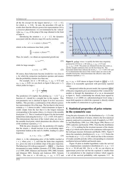
The prediction (23) implies that plotting (pt − 1/2) −2 as a
function of t should be a straight line in this regime. This
non-parametric test is checked in figure 8 on five successive
bubbles. This provides a confirmation of the effective powerlaw
representation (16) of the map. The fact that it is the lowest
estimate µ ≈ 3 shown in table 1 which dominates in figure 8
results simply from the fact that it is the longest transient
corresponding to the regime where p is closest to the unstable
fixed point 1/2. This is visualized in figure 8 by the horizontal
dashed lines indicating the levels p−1/2 = 0.05, 0.01 and 0.2.
This demonstrates that most of the visited values are close to
the unstable fixed point, which determines the effective value
of the nonlinear exponent µ ≈ 3.
With the price dynamics (8), the prediction (22) implies
that the returns rt should increase in an accelerating superexponential
fashion at the end of a bubble, leading to a price
trajectory
πt = πc − C(tc − t) µ(m)−2
µ(m)−1 , (24)
where πc is the culminating price of the bubble reached at
t = tc when µ(m) > 2, such that the finite-time singularity
in rt gives rise only to an infinite slope of the price trajectory.
The behaviour (24) with an exponent 0 < µ(m)−2
< 1 has been
µ(m)−1
documented in many bubbles (Sornette et al 1996, Johansen
et al 1999, 2000, Johansen and Sornette 1999, 2000, Sornette
and Johansen 2001, Sornette and Andersen 2001, Sornette
2001). The case m = 60 with ρhb = ρbh = 0.72 and
272
169
1
Figure 8. (pt −1/2) 2 versus t to qualify the finite-time singularity
predicted by (23) for m = 60 with ρhb = ρbh = 0.72 and
ρhh = ρbb = 0.85. The points are obtained from the time series pt
and the straight continuous lines are the best linear fits. The
horizontal dashed lines indicate the levels p − 1/2 = 0.05, 0.01 and
0.2 to demonstrate that most of the visited values are close to the
unstable fixed point, which determines the effective value of the
nonlinear exponent µ ≈ 3.
ρhh = ρbb = 0.85 shown in figure 6 leads to µ(m)−2
= 1/2,
µ(m)−1
which is in reasonable agreement with previously reported
values.
Interpreted within the present model, the exponent µ(m)−2
µ(m)−1
of the price singularity gives an estimation of the ‘connectivity’
number m through the dependence of µ on m documented
in figure 6. Such a relationship has already been argued by
Johansen et al (2000) at a phenomenological level using a
mean-field equation in which the exponent is directly related
to the number of connections to a given agent.
5. Statistical properties of price returns
in the symmetric case
Using the price dynamics (8), the distribution of p − 1/2 is the
same as the distribution of returns, which is the first statistical
property analysed in econometric work (Campbell et al 1997,
Lo and MacKinlay 1999, Lux 1996, Pagan 1996, Plerou et al
1999, Laherrère and Sornette 1998). Note that the distribution
of p − 1/2 is nothing but the invariant measure of the chaotic
map p ′ (p) which can be shown to be continuous with respect to
the Lebesgue measure (Eckmann and Ruelle 1985). Figure 9
shows the cumulative distribution of rt ∝ pt −1/2. Notice the
two breaks at |p − 1/2| =0.28, which are due to the existence
of weakly unstable periodic orbits corresponding to a transient
oscillation between bullish and bearish states.
Figure 10 plots in double-logarithmic scales the survival
(i.e. complementary cumulative) distribution of rt ∝ pt − 1/2
for m = 30, 60 and 100. For m = 60, we can observe an
approximate power-law tail but the exponent is smaller than
1 in contradiction to the empirical evidence which suggests
a tail of the survival probability with exponents 3–5. In