statistique, théorie et gestion de portefeuille - Docs at ISFA
statistique, théorie et gestion de portefeuille - Docs at ISFA
statistique, théorie et gestion de portefeuille - Docs at ISFA

Create successful ePaper yourself
Turn your PDF publications into a flip-book with our unique Google optimized e-Paper software.
12.2. Minimiser l’impact <strong>de</strong>s grands co-mouvements 383<br />
Cutting edge l<br />
Portfolio tail risk<br />
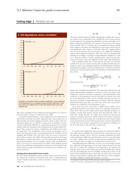
1. Tail <strong>de</strong>pen<strong>de</strong>nce versus correl<strong>at</strong>ion<br />
λ<br />
λ<br />
1.0<br />
0.9<br />
0.8<br />
0.7<br />
0.6<br />
0.5<br />
0.4<br />
0.3<br />
0.2<br />
0.1<br />
0<br />
–1.0 –0.8 –0.6 –0.4 –0.2 0<br />
ρ<br />
0.2 0.4 0.6 0.8 1.0<br />
1.0<br />
0.9<br />
0.8<br />
0.7<br />
0.6<br />
0.5<br />
0.4<br />
0.3<br />
0.2<br />
0.1<br />
Tail in<strong>de</strong>x ν = 3<br />
Tail in<strong>de</strong>x ν = 10<br />
0<br />
–1.0 –0.8 –0.6 –0.4 –0.2 0<br />
ρ<br />
0.2 0.4 0.6 0.8 1.0<br />
Evolution as a function of the correl<strong>at</strong>ion coefficient ρ of the coefficient<br />
of tail <strong>de</strong>pen<strong>de</strong>nce for an elliptical bivari<strong>at</strong>e Stu<strong>de</strong>nt distribution (solid<br />
line) and for the additive factor mo<strong>de</strong>l with Stu<strong>de</strong>nt factor and noise<br />
(dashed line)<br />
th<strong>at</strong> can be quantified by the coefficient of tail <strong>de</strong>pen<strong>de</strong>nce (for other d<strong>et</strong>ails,<br />
the rea<strong>de</strong>r is referred to Ledford & Tawn, 1998).<br />
For practical implement<strong>at</strong>ions, a direct applic<strong>at</strong>ion of the <strong>de</strong>finitions (1)<br />
and (2) fails to provi<strong>de</strong> reasonable estim<strong>at</strong>ions due to the double curse of<br />
dimensionality and un<strong>de</strong>r-sampling of extreme values, so th<strong>at</strong> a fully nonparam<strong>et</strong>ric<br />
approach is not reliable. It turns out to be possible to circumvent<br />
this fundamental difficulty by consi<strong>de</strong>ring the general class of factor<br />
mo<strong>de</strong>ls, which are among the most wi<strong>de</strong>spread and vers<strong>at</strong>ile mo<strong>de</strong>ls in finance.<br />
They come in two classes: multiplic<strong>at</strong>ive and additive factor mo<strong>de</strong>ls<br />
respectively. The multiplic<strong>at</strong>ive factor mo<strong>de</strong>ls are generally used to<br />
mo<strong>de</strong>l ass<strong>et</strong> fluctu<strong>at</strong>ions due to an un<strong>de</strong>rlying stochastic vol<strong>at</strong>ility (see, for<br />
example, Hull & White, 1987, and Taylor, 1994, for a survey of the properties<br />
of these mo<strong>de</strong>ls). The additive factor mo<strong>de</strong>ls are ma<strong>de</strong> to rel<strong>at</strong>e ass<strong>et</strong><br />
fluctu<strong>at</strong>ions to mark<strong>et</strong> fluctu<strong>at</strong>ions, as in the capital ass<strong>et</strong> pricing mo<strong>de</strong>l<br />
and its generalis<strong>at</strong>ions (see, for example, Sharpe, 1964, and Rubinstein,<br />
1973), or to any s<strong>et</strong> of common factors as in Ross’ (1976) arbitrage pricing<br />
theory. The coefficient of tail <strong>de</strong>pen<strong>de</strong>nce is known in closed form for both<br />
classes of factor mo<strong>de</strong>ls, which allows, as we shall see, for an efficient empirical<br />
estim<strong>at</strong>ion.<br />
Tail <strong>de</strong>pen<strong>de</strong>nce gener<strong>at</strong>ed by factor mo<strong>de</strong>ls<br />
We first examine multiplic<strong>at</strong>ive factor mo<strong>de</strong>ls, which account for most of<br />
the stylised facts observed on financial time series. A multivari<strong>at</strong>e stochastic<br />
vol<strong>at</strong>ility mo<strong>de</strong>l with a common stochastic vol<strong>at</strong>ility factor can be<br />
written as:<br />
130 RISK NOVEMBER 2002 ● WWW.RISK.NET<br />
where σ is a positive random variable mo<strong>de</strong>lling the vol<strong>at</strong>ility, Y is a Gaussian<br />
random vector, in<strong>de</strong>pen<strong>de</strong>nt of σ, and X is the vector of ass<strong>et</strong> r<strong>et</strong>urns.<br />
In this framework, the multivari<strong>at</strong>e distribution of ass<strong>et</strong> r<strong>et</strong>urns X is an elliptical<br />
multivari<strong>at</strong>e distribution. For instance, if the inverse of the square<br />
of the vol<strong>at</strong>ility 1/σ2 is a constant times a χ2-distributed random variable<br />
with ν <strong>de</strong>grees of freedom, the distribution of ass<strong>et</strong> r<strong>et</strong>urns will be the Stu<strong>de</strong>nt<br />
distribution with ν <strong>de</strong>grees of freedom. When the vol<strong>at</strong>ility follows<br />
Arch or Garch processes, the ass<strong>et</strong> r<strong>et</strong>urns are also elliptically distributed<br />
with f<strong>at</strong>-tailed marginal distributions. Thus, any ass<strong>et</strong> Xi is asymptotically<br />
distributed according to a regularly varying distribution1 : Pr{|Xi | > x} ~ L(x)<br />
× x –ν , where L(⋅) <strong>de</strong>notes a slowly varying function, with the same exponent<br />
ν for all ass<strong>et</strong>s, due to the ellipticity of their multivari<strong>at</strong>e distribution.<br />
Hult & Lindskog (2002) have shown th<strong>at</strong> the necessary and sufficient<br />
condition for any two ass<strong>et</strong>s Xi and Xj with an elliptical multivari<strong>at</strong>e distribution<br />
to have a non-vanishing coefficient of tail <strong>de</strong>pen<strong>de</strong>nce is th<strong>at</strong> their<br />
distribution be regularly varying. Denoting by ρij the correl<strong>at</strong>ion coefficient<br />
b<strong>et</strong>ween the ass<strong>et</strong>s Xi and Xj and by ν the tail in<strong>de</strong>x of their distributions,<br />
they obtain:<br />
π / 2<br />
ν<br />
∫<br />
dt cos t<br />
± ( π/ 2−arcsin ρij<br />
) / 2<br />
ν + 1<br />
λij<br />
= = 2I<br />
1+<br />
ρ ,<br />
π / 2<br />
ij<br />
(4)<br />
ν<br />
dt cos t<br />
2 2<br />
1 ⎛ ⎞<br />
⎝<br />
⎜<br />
2⎠<br />
⎟<br />
where the function:<br />
∫<br />
0<br />
X =σY<br />
1<br />
Ix( z, w)=<br />
Bzw ( , )<br />
( )<br />
x z−1<br />
w−1<br />
dt t 1 − t<br />
0<br />
<strong>de</strong>notes the incompl<strong>et</strong>e b<strong>et</strong>a function. This expression holds for any regularly<br />
varying elliptical distribution, irrespective of the exact shape of the<br />
distribution. Only the tail in<strong>de</strong>x is important in the d<strong>et</strong>ermin<strong>at</strong>ion of the<br />
coefficient of tail <strong>de</strong>pen<strong>de</strong>nce because λ ± ij probes the extreme end of the<br />
tail of the distributions, which all have, roughly speaking, the same behaviour<br />
for regularly varying distributions. In contrast, when the marginal<br />
distributions <strong>de</strong>cay faster than any power law, such as the Gaussian distribution,<br />
the coefficient of tail <strong>de</strong>pen<strong>de</strong>nce is zero.<br />
L<strong>et</strong> us now turn to the second class of additive factor mo<strong>de</strong>ls, whose<br />
introduction in finance goes back <strong>at</strong> least to the arbitrage pricing theory<br />
(Ross, 1976). They are now wi<strong>de</strong>ly used in many branches of finance, including<br />
to mo<strong>de</strong>l stock r<strong>et</strong>urns, interest r<strong>at</strong>es and credit risks. Here, we<br />
shall only consi<strong>de</strong>r the effect of a single factor, which may represent the<br />
mark<strong>et</strong>, for example. This factor will be <strong>de</strong>noted by Y and its cumul<strong>at</strong>ive<br />
distribution by FY . As previously, the vector X is the vector of ass<strong>et</strong> r<strong>et</strong>urns<br />
and ε will <strong>de</strong>note the vector of idiosyncr<strong>at</strong>ic noises assumed in<strong>de</strong>pen<strong>de</strong>nt2 of Y. β is the vector whose components are the regression coefficients of<br />
the Xi on the factor Y. Thus, the factor mo<strong>de</strong>l reads:<br />
(6)<br />
In contrast with multiplic<strong>at</strong>ive factor mo<strong>de</strong>ls, the multivari<strong>at</strong>e distribution<br />
of X cannot be obtained in an analytical form, in the general case. In<br />
the particular situ<strong>at</strong>ion when Y and ε are normally distributed, the multivari<strong>at</strong>e<br />
distribution of X is also normal but this case is not very interesting.<br />
In a sense, additive factor mo<strong>de</strong>ls are richer than the multiplic<strong>at</strong>ive ones,<br />
since they give birth to a larger s<strong>et</strong> of distributions of ass<strong>et</strong> r<strong>et</strong>urns.<br />
Notwithstanding these difficulties, it turns out to be possible to obtain<br />
the coefficient of tail <strong>de</strong>pen<strong>de</strong>nce for any pair of ass<strong>et</strong>s Xi and Xj . In a first<br />
step, l<strong>et</strong> us consi<strong>de</strong>r the coefficient of tail <strong>de</strong>pen<strong>de</strong>nce λ ± i b<strong>et</strong>ween any<br />
ass<strong>et</strong> Xi and the factor Y itself. Malevergne & Sorn<strong>et</strong>te (2002b) have shown<br />
th<strong>at</strong> λ ± X = βY+ ε<br />
i is also i<strong>de</strong>ntically zero for all rapidly varying factors, th<strong>at</strong> is, for all<br />
factors whose distribution <strong>de</strong>cays faster than any power law, such as the<br />
Gaussian, exponential or gamma laws. When the factor Y has a distribution<br />
th<strong>at</strong> is regularly varying with tail in<strong>de</strong>x ν, we have:<br />
1 See Bingham, Goldie & Teugel (1987) for d<strong>et</strong>ails on regular vari<strong>at</strong>ions<br />
2 In fact, ε and Y can be weakly <strong>de</strong>pen<strong>de</strong>nt (see Malevergne & Sorn<strong>et</strong>te, 2002b, for d<strong>et</strong>ails)<br />
∫<br />
(3)<br />
(5)