statistique, théorie et gestion de portefeuille - Docs at ISFA
statistique, théorie et gestion de portefeuille - Docs at ISFA
statistique, théorie et gestion de portefeuille - Docs at ISFA

Create successful ePaper yourself
Turn your PDF publications into a flip-book with our unique Google optimized e-Paper software.
384 12. Gestion <strong>de</strong>s risques grands <strong>et</strong> extrêmes<br />
where:<br />
λ<br />
+<br />
i =<br />
l =<br />
A similar expression holds for λ – i , which is obtained by simply replacing<br />
the limit u → 1 by u → 0 in the <strong>de</strong>finition of l. λ ± i is non-zero as long<br />
as l remains finite, th<strong>at</strong> is, when the tail of the distribution of the factor is<br />
not thinner than the tail of the idiosyncr<strong>at</strong>ic noise εi . Therefore, two conditions<br />
must hold for the coefficient of tail <strong>de</strong>pen<strong>de</strong>nce to be non-zero:<br />
the factor must be intrinsically ‘wild’ (to use the terminology of Man<strong>de</strong>lbrot,<br />
1997) so th<strong>at</strong> its distribution is regularly varying; and<br />
the factor must be sufficiently ‘wild’ in its intrinsic variability, so th<strong>at</strong> its<br />
influence is not domin<strong>at</strong>ed by the idiosyncr<strong>at</strong>ic component of the ass<strong>et</strong>.<br />
Then, the amplitu<strong>de</strong> of λ ± i is d<strong>et</strong>ermined by the tra<strong>de</strong>-off b<strong>et</strong>ween the rel<strong>at</strong>ive<br />
tail behaviours of the factor and the idiosyncr<strong>at</strong>ic noise.<br />
As an example, l<strong>et</strong> us consi<strong>de</strong>r th<strong>at</strong> the factor and the idiosyncr<strong>at</strong>ic noise<br />
follow Stu<strong>de</strong>nt distribution with νY and ν <strong>de</strong>grees of freedom and scale<br />
εi<br />
factor σY and σ respectively. Expression (7) leads to:<br />
εi<br />
λi = 0 if νY > νεi<br />
λi =<br />
1<br />
1<br />
σεi<br />
ν<br />
if νY = νε= ν<br />
i<br />
+ ( βσ i Y)<br />
−1<br />
lim<br />
u→1<br />
Y<br />
ν<br />
l { 1 β } i<br />
( )<br />
( )<br />
FXu −1<br />
F u<br />
λ = 1 if ν < ν<br />
i Y<br />
The tail <strong>de</strong>pen<strong>de</strong>nce <strong>de</strong>creases when the idiosyncr<strong>at</strong>ic vol<strong>at</strong>ility increases<br />
rel<strong>at</strong>ive to the factor vol<strong>at</strong>ility. Therefore, λi <strong>de</strong>creases in periods<br />
of high idiosyncr<strong>at</strong>ic vol<strong>at</strong>ility and increases in periods of high mark<strong>et</strong><br />
vol<strong>at</strong>ility. From the viewpoint of the tail <strong>de</strong>pen<strong>de</strong>nce, the vol<strong>at</strong>ility of an<br />
ass<strong>et</strong> is not relevant. Wh<strong>at</strong> is governing extreme co-movement is the rel<strong>at</strong>ive<br />
weights of the different components of the vol<strong>at</strong>ility of the ass<strong>et</strong>.<br />
Figure 1 compares the coefficient of tail <strong>de</strong>pen<strong>de</strong>nce as a function of<br />
the correl<strong>at</strong>ion coefficient for the bivari<strong>at</strong>e Stu<strong>de</strong>nt distribution (expression<br />
(4)) and for the factor mo<strong>de</strong>l with the factor and the idiosyncr<strong>at</strong>ic noise<br />
following Stu<strong>de</strong>nt distributions (equ<strong>at</strong>ion (8)). Contrary to the coefficient<br />
of tail <strong>de</strong>pen<strong>de</strong>nce of the Stu<strong>de</strong>nt factor mo<strong>de</strong>l, the tail <strong>de</strong>pen<strong>de</strong>nce of the<br />
(elliptical) Stu<strong>de</strong>nt distribution does not vanish for neg<strong>at</strong>ive correl<strong>at</strong>ion coefficients.<br />
For large values of the correl<strong>at</strong>ion coefficient, the former is always<br />
larger than the l<strong>at</strong>ter.<br />
Once the coefficients of tail <strong>de</strong>pen<strong>de</strong>nce b<strong>et</strong>ween the ass<strong>et</strong>s and the<br />
common factor are known, the coefficient of tail <strong>de</strong>pen<strong>de</strong>nce b<strong>et</strong>ween any<br />
two ass<strong>et</strong>s Xi and Xj with a common factor Y is simply equal to the weakest<br />
tail <strong>de</strong>pen<strong>de</strong>nce b<strong>et</strong>ween the ass<strong>et</strong>s and their common factor:<br />
λ min λ , λ<br />
(9)<br />
= { }<br />
ij i j<br />
This result is very intuitive: since the <strong>de</strong>pen<strong>de</strong>nce b<strong>et</strong>ween the two ass<strong>et</strong>s<br />
is due to their common factor, this <strong>de</strong>pen<strong>de</strong>nce cannot be stronger than<br />
the weakest <strong>de</strong>pen<strong>de</strong>nce b<strong>et</strong>ween each of the ass<strong>et</strong>s and the factor.<br />
Practical implement<strong>at</strong>ion and consequences<br />
The two m<strong>at</strong>hem<strong>at</strong>ical results (4) and (7) have a very important practical<br />
effect for estim<strong>at</strong>ing the coefficient of tail <strong>de</strong>pen<strong>de</strong>nce. As we have already<br />
pointed out, its direct estim<strong>at</strong>ion is essentially impossible since, by <strong>de</strong>finition,<br />
the number of observ<strong>at</strong>ions goes to zero as the probability level of<br />
the quantile goes to zero (or one). In contrast, the formulas (4) and (7–9)<br />
tell us th<strong>at</strong> one has just to estim<strong>at</strong>e a tail in<strong>de</strong>x and a correl<strong>at</strong>ion coefficient.<br />
These estim<strong>at</strong>ions can be reasonably accur<strong>at</strong>e because they make<br />
use of a significant part of the d<strong>at</strong>a beyond the few extremes targ<strong>et</strong>ed by<br />
λ. Moreover, equ<strong>at</strong>ion (7) does not explicitly assume a power law behaviour,<br />
but only a regularly varying behaviour, which is far more general. In<br />
1<br />
max ,<br />
εi<br />
(7)<br />
(8)<br />
A. Coefficients of tail <strong>de</strong>pen<strong>de</strong>nce<br />
Lower tail <strong>de</strong>pen<strong>de</strong>nce Upper tail <strong>de</strong>pen<strong>de</strong>nce<br />
Bristol-Myers Squibb 0.16 (0.03) 0.14 (0.01)<br />
Chevron 0.05 (0.01) 0.03 (0.01)<br />
Hewl<strong>et</strong>t-Packard 0.13 (0.01) 0.12 (0.01)<br />
Coca-Cola 0.12 (0.01) 0.09 (0.01)<br />
Minnesota Mining & MFG 0.07 (0.01) 0.06 (0.01)<br />
Philip Morris 0.04 (0.01) 0.04 (0.01)<br />
Procter & Gamble 0.12 (0.02) 0.09 (0.01)<br />
Pharmacia 0.06 (0.01) 0.04 (0.01)<br />
Schering-Plough 0.12 (0.01) 0.11 (0.01)<br />
Texaco 0.04 (0.01) 0.03 (0.01)<br />
Texas Instruments 0.17 (0.02) 0.12 (0.01)<br />
Walgreen 0.11 (0.01) 0.09 (0.01)<br />
This table presents the coefficients of lower and upper tail <strong>de</strong>pen<strong>de</strong>nce with the S&P<br />
500 in<strong>de</strong>x for a s<strong>et</strong> of 12 major stocks tra<strong>de</strong>d on the New York Stock Exchange from<br />
January 1991 to December 2000. The numbers in brack<strong>et</strong>s give the estim<strong>at</strong>ed standard<br />
<strong>de</strong>vi<strong>at</strong>ion of the empirical coefficients of tail <strong>de</strong>pen<strong>de</strong>nce<br />
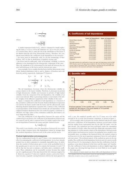
2. Quantile r<strong>at</strong>io<br />
I = X k,N /Y k,N<br />
2.2<br />
2.0<br />
1.8<br />
1.6<br />
1.4<br />
1.2<br />
1.0<br />
0.8<br />
0 0.05 0.10 0.15 0.20 0.25<br />
k/N<br />
^<br />
Empirical estim<strong>at</strong>e l of the quantile r<strong>at</strong>io l in (7) versus the empirical<br />
^<br />
quantile k/N. We observe a very good stability of l for quantiles<br />
ranging b<strong>et</strong>ween 0.005 and 0.05<br />
such a case, the empirical quantile r<strong>at</strong>io l in (7) turns out to be stable<br />
enough for its accur<strong>at</strong>e non-param<strong>et</strong>ric estim<strong>at</strong>ion, as shown in figure 2.<br />
As an example, table A presents the results obtained both for the upper<br />
and lower coefficients of tail <strong>de</strong>pen<strong>de</strong>nce b<strong>et</strong>ween several major stocks<br />
and the mark<strong>et</strong> factor represented here by the S&P 500 in<strong>de</strong>x, over the<br />
past <strong>de</strong>ca<strong>de</strong>. The estim<strong>at</strong>ion has been performed un<strong>de</strong>r the assumption<br />
th<strong>at</strong> equ<strong>at</strong>ion (6) holds, r<strong>at</strong>her than un<strong>de</strong>r the ellipticality assumption yielding<br />
equ<strong>at</strong>ion (4). In the present context of the <strong>de</strong>pen<strong>de</strong>nce b<strong>et</strong>ween stocks<br />
and an in<strong>de</strong>x (not b<strong>et</strong>ween two stocks), favouring the factor mo<strong>de</strong>l is very<br />
reasonable since, according to the financial theory, the mark<strong>et</strong>’s r<strong>et</strong>urn is<br />
well known to be the most important explan<strong>at</strong>ory factor for each individual<br />
ass<strong>et</strong> r<strong>et</strong>urn. 3 The technical aspects of the m<strong>et</strong>hod are given in the Appendix.<br />
The coefficient of tail <strong>de</strong>pen<strong>de</strong>nce b<strong>et</strong>ween any two ass<strong>et</strong>s is easily<br />
<strong>de</strong>rived from (9). It is interesting to observe th<strong>at</strong> the coefficients of tail <strong>de</strong>pen<strong>de</strong>nce<br />
seem almost i<strong>de</strong>ntical in the lower and the upper tail. Non<strong>et</strong>heless,<br />
the coefficient of lower tail <strong>de</strong>pen<strong>de</strong>nce is always slightly larger than<br />
the upper one, showing th<strong>at</strong> large losses are more likely to occur tog<strong>et</strong>her<br />
than large gains.<br />
Two clusters of ass<strong>et</strong>s stand out: those with a tail <strong>de</strong>pen<strong>de</strong>nce of about<br />
3 In a situ<strong>at</strong>ion where the common factor cannot be easily i<strong>de</strong>ntified or estim<strong>at</strong>ed, the<br />
ellipticality assumption may provi<strong>de</strong> a useful altern<strong>at</strong>ive<br />
WWW.RISK.NET ● NOVEMBER 2002 RISK 131