statistique, théorie et gestion de portefeuille - Docs at ISFA

12.2. Minimiser l’impact des grands co-mouvements 385
Cutting edge l
Portfolio tail risk
3. Portfolios versus market
Portfolio daily return
0.10
0.08
0.06
0.04
0.02
0
0.02
0.04
0.06
0.08
Portfolio 1
Linear regression of
the portfolio 1 on the
S&P 500 index
Portfolio 2
Linear regression of
the portfolio 2 on the
S&P 500 index
0.10
0.08 0.06 0.04 0.02 0 0.02 0.04 0.06
S&P 500 daily return
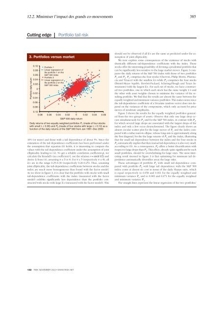
Daily returns of two equally weighted portfolios P 1 (made of four stocks
with small λ ≤ 0.06) and P 2 (made of four stocks with large λ ≥ 0.12) as a
function of the daily returns of the S&P 500 from Jan 1991–Dec 2000
10% (or more) and those with a tail dependence of about 5%. Since the
estimation of the tail dependence coefficients has been performed under
the assumption that equation (6) holds, it is interesting to compare the
values with the tail dependence coefficient under the assumption of joint
ellipticality leading to (4). To get a reliable correlation coefficient ρ, we
calculate the Kendall’s tau coefficient τ, use the relation r = sin(πτ/2) and
derive λ from (4), assuming ν = 3 or 4. For ν = 3 (respectively ν = 4), all
λ’s are in the range 0.25–0.30 (respectively 0.20–0.25). Thus, assuming
joint ellipticality, the tail-dependence coefficients between stocks and the
index are much more homogeneous than found with the factor model.
As we show in figure 3, it is clear that the portfolio with stocks with small
tail-dependence coefficients with the index (measured with the factor
model) exhibits significantly less dependence than the portfolio constructed
with stocks with large λ’s (measured with the factor model). This
132 RISK NOVEMBER 2002 ● WWW.RISK.NET
should not be observed if all λ’s are the same as predicted under the assumption
of joint ellipticality.
We now explore some consequences of the existence of stocks with
drastically different tail-dependence coefficients with the index. These
stocks offer the interesting possibility of devising a prudential portfolio that
can be significantly less sensitive to the large market moves. Figure 3 compares
the daily returns of the S&P 500 index with those of two portfolios
P 1 and P 2 . P 1 comprises the four stocks (Chevron, Philip Morris, Pharmacia
and Texaco) with the smallest λ’s while P 2 comprises the four stocks
(Bristol-Meyer Squibb, Hewlett-Packard, Schering-Plough and Texas Instruments)
with the largest λ’s. For each set of stocks, we have constructed
two portfolios, one in which each stock has the same weight 1/4 and
the other with asset weights chosen to minimise the variance of the resulting
portfolio. We find that the results are almost the same between the
equally weighted and minimum-variance portfolios. This makes sense since
the tail-dependence coefficient of a bivariate random vector does not depend
on the variances of the components, which only account for price
moves of moderate amplitudes.
Figure 3 shows the results for the equally weighted portfolios generated
from the two groups of assets. Observe that only one large drop occurs
simultaneously for P 1 and for the S&P 500 index, in contrast with P 2 ,
for which several large drops are associated with the largest drops of the
index and only a few occur desynchronised. The figure clearly shows an
almost circular scatter plot for the large moves of P 1 and the index compared
with a rather narrow ellipse, whose long axis is approximately along
the first diagonal, for the the large returns of P 2 and the index, illustrating
that the small tail dependence between the index and the four stocks in
P 1 automatically implies that their mutual tail dependence is also very small,
according to (9). As a consequence, P 1 offers a better diversification with
respect to large drops than P 2 . This effect, already quite significant for such
small portfolios, should be overwhelming for large ones. The most interesting
result stressed in figure 3 is that optimising for minimum tail dependence
automatically diversifies away the large risks.
These advantages of portfolio P 1 with small tail dependence compared
with portfolio P 2 with large tail dependence with the S&P 500
index come at almost no cost in terms of the daily Sharpe ratio, which
is equal respectively to 0.058 and 0.061 for the equally weighted and
minimum variance P 1 and to 0.069 and 0.071 for the equally weighted
and minimum variance P 2 .
The straight lines represent the linear regression of the two portfolios’