Numerical Methods Contents - SAM

(Linear) generalized eigenvalue problem:
Given A ∈ C n,n , regular B ∈ C n,n , seek x ≠ 0, λ ∈ C
Ax = λBx ⇔ B −1 Ax = λx . (5.1.3)
x ˆ= generalized eigenvector, λ ˆ= generalized eigenvalue
Obviously every generalized eigenvalue problem is equivalent to a standard eigenvalue problem
Ax = λBx ⇔ B −1 A = λx .
QR-algorithm (with shift)
in general: quadratic convergence
cubic convergence for normal
matrices
(→ [18, Sect. 7.5,8.2])
Code 5.2.2: QR-algorithm with shift
1 function d = e i g q r (A, t o l )
2 n = size (A, 1 ) ;
3 while (norm( t r i l (A,−1) ) > t o l ∗norm(A) )
4 s h i f t = A( n , n ) ;
5 [Q,R] = qr ( A − s h i f t ∗ eye ( n ) ) ;
6 A = Q’∗A∗Q;
7 end
8 d = diag (A) ;
However, usually it is not advisable to use this equivalence for numerical purposes!
Computational cost:
O(n 3 ) operations per step of the QR-algorithm
Remark 5.1.1 (Generalized eigenvalue problems and Cholesky factorization).
If B = B H s.p.d. (→ Def. 2.7.1) with Cholesky factorization B = R H R
Ax = λBx ⇔ Ãy = λy where à := R−H AR −1 , y := Rx .
★
✧
Library implementations of the QR-algorithm provide numerically stable
eigensolvers (→ Def.2.5.5)
✥
✦
➞
This transformation can be used for efficient computations.
△
Ôº¼½ º¾
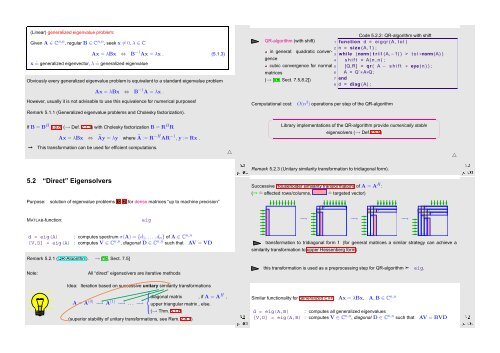
Remark 5.2.3 (Unitary similarity transformation to tridiagonal form).
△
Ôº¼¿ º¾
5.2 “Direct” Eigensolvers
Successive Householder similarity transformations of A = A H :
(➞ ˆ= affected rows/columns, ˆ= targeted vector)
Purpose:
solution of eigenvalue problems ➊, ➋ for dense matrices “up to machine precision”
0 0
0 0
0 0
0
0
0
0
MATLAB-function:
eig
−→
0
−→
0
0
−→
0
0
0
0
0
d = eig(A) : computes spectrum σ(A) = {d 1 ,...,d n } of A ∈ C n,n
[V,D] = eig(A) : computes V ∈ C n,n , diagonal D ∈ C n,n such that AV = VD
Remark 5.2.1 (QR-Algorithm). → [18, Sect. 7.5]
Note:
All “direct” eigensolvers are iterative methods
0
0 0
0 0 0
transformation to tridiagonal form ! (for general matrices a similar strategy can achieve a
similarity transformation to upper Hessenberg form)
this transformation is used as a preprocessing step for QR-algorithm ➣ eig.
△
Idea: Iteration based on successive unitary similarity transformations
⎧
⎪⎨ diagonal matrix , if A = A H ,
A = A (0) −→ A (1) −→ ... −→ upper triangular matrix , else.
⎪⎩
(→ Thm. 5.1.6)
(superior stability of unitary transformations, see Rem. 2.8.1)
Ôº¼¾ º¾
Ôº¼ º¾
[V,D] = eig(A,B) : computes V ∈ C n,n , diagonal D ∈ C n,n such that AV = BVD
Similar functionality for generalized EVP Ax = λBx, A,B ∈ C n,n
d = eig(A,B)
: computes all generalized eigenvalues