Numerical Methods Contents - SAM

✬
Theorem 5.5.7 (best low rank approximation).
Let A = UΣV H be the SVD of A ∈ K m.n (→ Thm. 5.5.1). For 1 ≤ k ≤ rank(A) set U k :=
[
u·,1 , ...,u·,k
]
∈ K m,k , Vk := [ v·,1 ,...,v·,k
]
∈ K n,k , Σk := diag(σ 1 ,...,σ k ) ∈ K k,k .
Then, for ‖·‖ = ‖·‖ F and ‖·‖ = ‖·‖ 2 , holds true
∥
∥A − U k Σ k Vk
H ∥ ≤ ‖A − F‖ ∀F ∈ R k (m, n) .
✫
✩
✪
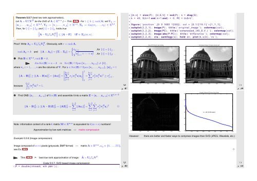
2 [m, n ] = size (P) ; [U, S, V] = svd (P) ; s = diag (S) ;
3 k = 40; S( k +1:end , k +1:end ) = 0 ; PC = U∗S∗V ’ ;
4
5 figure ( ’ p o s i t i o n ’ , [ 0 0 1600 1200]) ; c o l = [ 0 : 1 / 2 1 5 : 1 ] ’ ∗ [ 1 , 1 , 1 ] ;
6 subplot ( 2 , 2 , 1 ) ; image (P) ; t i t l e ( ’ o r i g i n a l image ’ ) ; colormap ( c o l ) ;
7 subplot ( 2 , 2 , 2 ) ; image (PC) ; t i t l e ( ’ compressed (40 S .V . ) ’ ) ; colormap ( c o l ) ;
8 subplot ( 2 , 2 , 3 ) ; image ( abs (P−PC) ) ; t i t l e ( ’ d i f f e r e n c e ’ ) ; colormap ( c o l ) ;
9 subplot ( 2 , 2 , 4 ) ; cla ; semilogy ( s ) ; hold on ; plot ( k , s ( k ) , ’ ro ’ ) ;
Proof. Write A k = U k Σ k Vk H . Obviously, with r = rankA,
View of ETH Zurich main building
Compressed image, 40 singular values used
rankA k = k and ‖A − A k ‖ = ‖Σ − Σ k ‖ =
{
√ σk+1 , for ‖·‖ = ‖·‖ 2 ,
σk+1 2 + · · · + σ2 r , for ‖·‖ = ‖·‖ F .
100
200
100
200
➊ Pick B ∈ K n,n , rankB = k.
dim Ker(B) = n − k ⇒ Ker(B) ∩ Span {v 1 ,...,v k+1 } ≠ {0} ,
where v i , i = 1,...,n are the columns of V. For x ∈ Ker(B) ∩ Span {v 1 ,...,v k+1 }, ‖x‖ 2 = 1
∥ ∥∥∥∥∥
‖A − B‖ 2 k+1
2 ≥ ‖(A − B)x‖2 2 = ‖Ax‖2 2 = ∑
2
σ j (vj H x)u k+1 ∑
j
= σj 2
j=1 ∥
(vH j x)2 ≥ σj+1 2 ,
2 j=1
k+1 ∑
because
Ôº º
j
j=1(v Hx)2 = 1.
300
400
500
600
700
800
200 400 600 800 1000 1200
300
400
500
600
700
Ôº º
800
200 400 600 800 1000 1200
➋
Find ONB {z 1 , ...,z n−k } of Ker(B) and assemble it into a matrix Z = [z 1 ...z n−k ] ∈ K n,n−k
Difference image: |original − approximated|
Singular Values of ETH view (Log−Scale)
10 6 k = 40 (0.08 mem)
100
10 5
‖A − B‖ 2 n−k
F ≥ ‖(A − B)Z‖2 F = ‖AZ‖2 F = ∑
‖Az i ‖ 2 n−k
2 = ∑
i=1
i=1 j=1
r∑
σj 2 (vH j z i) 2
✷
200
300
400
10 4
10 3
500
10 2
600
Note: information content of a rank-k matrix M ∈ K m,n is equivalent to k(m + n) numbers!
700
10 1
Approximation by low-rank matrices ↔ matrix compression
800
200 400 600 800 1000 1200
10 0
0 100 200 300 400 500 600 700 800
Example 5.5.6 (Image compression).
However:
there are better and faster ways to compress images than SVD (JPEG, Wavelets, etc.)
Image composed of m×n pixels (greyscale, BMP format) ↔ matrixA ∈ R m,n , a ij ∈ {0, ...,255},
see Ex. 5.3.9
Ôº º
1 P = double ( imread ( ’ eth .pbm ’ ) ) ;
Thm. 5.5.7 ➣ best low rank approximation of image: Ã = U k Σ k V T
Code 5.5.7: SVD based image compression
✸
Ôº¼¼ º