Numerical Methods Contents - SAM

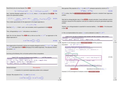
Recall that by the min-max theorem Thm. 5.3.5
u n = argmax x∈R n ρ A (x) , u n−1 = argmax x∈R n ,x⊥u n
ρ A (x) . (5.3.20)
Idea: maximize Rayleigh quotient over Span {v,w}, where v, w are output by Code 5.3.19. This
leads to the optimization problem
(α ∗ ,β ∗ ) := argmax ρ A (αv + βw) =
α,β∈R, α 2 +β 2 =1
( α
argmax ρ (v,w)
α,β∈R, α 2 +β 2 T A(v,w) ( =1 β
Then a better approximation for the eigenvector to the largest eigenvalue is
v ∗ := α ∗ v + β ∗ w .
Note that ‖v ∗ ‖ 2 = 1, if both v and w are normalized, which is guaranteed in Code 5.3.19.
Then, orthogonalizing w w.r.t v ∗ will produce a new iterate w ∗ .
)
) . (5.3.21)
More general: Ritz projection of Ax = λx onto Im(V) (subspace spanned by columns of V)
V H AVw = λV H Vw . (5.3.23)
If V is unitary, then this generalized eigenvalue problem will become a standard linear eigenvalue
problem.
Note that he orthogonalization step in Code 5.3.21 is actually redundant, if exact arithmetic could be
employed, because the Ritz projection could also be realized by solving the generalized eigenvalue
problem
However, prior orthogonalization is essential for numerical stability (→ Def. 2.5.5), cf. the discussion
in Sect. 2.8.
In MATLAB-implementations the vectors v, w can be collected in a matrix V ∈ R n,2 :
Again the min-max theorem Thm. 5.3.5 tells us that we can find (α ∗ , β ∗ ) T as eigenvector to the
largest eigenvalue of
( (
(v,w) T α α
A(v,w) = λ
β)
β)
Ôº¿ º¿
. (5.3.22)
Since eigenvectors of symmetric matrices are mutually orthogonal, we find w ∗ = α 2 v + β 2 w, where
(α 2 , β 2 ) T is the eigenvector of (5.4.1) belonging to the smallest eigenvalue. This assumes orthonormal
vectors v, w.
Summing up the following MATLAB-function performs these computations:
Code 5.3.22: one step of subspace power iteration, m = 2, with Ritz projection
1 function [ v ,w] = sspowitsteprp (A, v ,w)
2 v = A∗v ; w = A∗w; [Q,R] = qr ( [ v ,w] , 0 ) ; [U,D] = eig (Q’∗A∗Q) ;
3 ev = diag (D) ; [dummy, i d x ] = sort ( abs ( ev ) ) ;
4 w = Q∗U( : , i d x ( 1 ) ) ; v = Q∗U( : , i d x ( 2 ) ) ;
Code 5.3.23: one step of subspace power iteration with Ritz projection, matrix version
1 function V = sspowitsteprp (A,V)
2 V = A∗V ; [Q,R] = qr (V, 0 ) ; [U,D] = eig (Q’∗A∗Q) ; V = Q∗U;
Algorithm 5.3.24 (Subspace variant of direct power method with Ritz projection).
Assumption:
A = A H ∈ K n,n , k ≪ n
MATLAB-CODE : Subspace variant of direct power method for s.p.d. A
function [V,ev] = spowit(A,k,m,maxit)
n = size(A,1); V = rand(n,m); d = zeros(k,1);
for i=1:maxit
V=A*V;
[Q,R] = qr(V,0) ;
T=Q’*A*Q;
[S,D] = eig(T); [l,perm] = sort(-abs(diag(D)));
V = Q*S(:,perm);
if (norm(d+l(1:k)) < tol), break; end;
d = -l(1:k);
end
V = V(:,1:k); ev = diag(D(perm(1:k),perm(1:k)));
(5.3.24)
Ôº º¿
General technique:
Ritz projection
= “projection of a (symmetric) eigenvalue problem onto a subspace”
Example: Ritz projection of Ax = λx onto Span {v,w}:
( (
(v,w) T α
A(v,w) = λ(v,w)
β)
T α
(v,w)
β)
Ôº º¿
.
Ritz projection Generalized normalization to ‖z‖ 2 = 1
Example 5.3.25 (Convergence of subspace variant of direct power method).
Ôº º¿