Numerical Methods Contents - SAM

x (0) = 0 ➣ r 0 = e n ➣ K l (A,r 0 ) = Span {e n ,e n−1 ,...,e n−l+1 }
{
min{‖y − x‖ 2 : y ∈ K l (A,r 0 )} =
1 , if l ≤ n ,
0 , for l = n .
✸
Advantages of Krylov methods vs. direct elimination (, IF they converge at all/sufficiently fast).
• They require system matrix A in procedural form y=evalA(x) ↔ y = Ax only.
• They can perfectly exploit sparsity of system matrix.
• They can cash in on low accuracy requirements (, IF viable termination criterion available).
✗
✖
TRY
& PRAY
✔
✕
• They can benefit from a good initial guess.
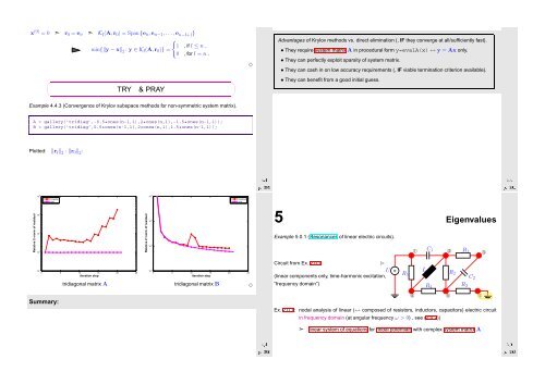
Example 4.4.3 (Convergence of Krylov subspace methods for non-symmetric system matrix).
A = gallery(’tridiag’,-0.5*ones(n-1,1),2*ones(n,1),-1.5*ones(n-1,1));
B = gallery(’tridiag’,0.5*ones(n-1,1),2*ones(n,1),1.5*ones(n-1,1));
Plotted: ‖r l ‖ 2 : ‖r 0 ‖ 2 :
Ôº¿ º
Ôº¿½ º
bicgstab
qmr
bicgstab
qmr
Relative 2−norm of residual
10 3 iteration step
10 2
10 1
10 0
10 −1
0 5 10 15 20 25
tridiagonal matrix A
Relative 2−norm of residual
10 0 iteration step
10 −1
10 −2
10 −3
0 5 10 15 20 25
tridiagonal matrix B ✸
5 Eigenvalues
Example 5.0.1 (Resonances of linear electric circuits).
➀
C 1 ➁ R 1 ➂
Circuit from Ex. 2.0.1
✄
U ~ L
R R 2
(linear components only, time-harmonic excitation, 5 C 2
“frequency domain”)
R4 R 3
Summary:
➃ ➄ ➅
Ex. 2.0.1: nodal analysis of linear (↔ composed of resistors, inductors, capacitors) electric circuit
in frequency domain (at angular frequency ω > 0) , see (2.0.2))
Fig. 55
Ôº¿¼ º
➣
linear system of equations for nodal potentials with complex system matrix A
Ôº¿¾ º¼