

Numerical Methods Contents - SAM
Numerical Methods Contents - SAM
Numerical Methods Contents - SAM

Create successful ePaper yourself
Turn your PDF publications into a flip-book with our unique Google optimized e-Paper software.
Mapping a ∈ K n to a multiple of e 1 by n − 1 successive Givens rotations:<br />
⎛<br />
⎛ ⎞ ⎛<br />
a 1<br />
a (1) ⎞<br />
a (2) ⎞<br />
⎛<br />
.<br />
1 1 a (n−1) ⎞<br />
G ⎜ .<br />
12 (a 1 ,a 2 )<br />
0 G<br />
⎟ −−−−−−−→<br />
⎜ a 13 (a (1)<br />
0 1 1 ,a 3)<br />
3 ⎟ −−−−−−−−→<br />
0<br />
G 14 (a (2)<br />
1 ,a 4) G 1n (a (n−2)<br />
0 1 ,a n )<br />
⎝ . ⎠ ⎝ . ⎠ ⎜ a −−−−−−−−→ · · · −−−−−−−−−−→<br />
.<br />
4 ⎟<br />
⎜ ⎟<br />
⎝<br />
a . ⎠<br />
⎝ . ⎠<br />
n a n<br />
a n 0<br />
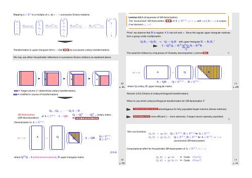
Transformation to upper triangular form (→ Def. 2.2.1) by successive unitary transformations:<br />
We may use either Householder reflections or successive Givens rotations as explained above.<br />
✬<br />
Lemma 2.8.3 (Uniqueness of QR-factorization).<br />
The “economical” QR-factorization (2.8.4) of A ∈ K m,n , m ≥ n, with rank(A) = n is unique,<br />
if we demand r ii > 0.<br />
✫<br />
Proof. we observe that R is regular, if A has full rank n. Since the regular upper triangular matrices<br />
form a group under multiplication:<br />
Q 1 R 1 = Q 2 R 2 ⇒ Q 1 = Q 2 R with upper triangular R := R 2 R −1<br />
1 .<br />
I = Q H 1 Q 1 = R H Q<br />
} H 2{{ Q } 2 R = R H R .<br />
=I<br />
The assertion follows by uniqueness of Cholesky decomposition, Lemma 2.7.6.<br />
✩<br />
✪<br />
✷<br />
⎛<br />
⎜<br />
⎝<br />
⎞ ⎛<br />
⎟<br />
⎠ ➤ ⎜<br />
⎝ 0 *<br />
⎞ ⎛<br />
⎟<br />
⎠ ➤ ⎜<br />
⎝ 0 *<br />
⎞ ⎛<br />
⎟<br />
⎠ ➤ ⎜<br />
⎝ 0 *<br />
⎞<br />
⎟<br />
⎠ .<br />
Ôº¾¼½ ¾º<br />
⎛<br />
⎞ ⎛ ⎞⎛<br />
m < n: ⎜ A<br />
⎟<br />
⎝<br />
⎠ = ⎜ Q<br />
⎟⎜<br />
⎝ ⎠⎝<br />
A = QR , Q ∈ K m,m , R ∈ K m,n ,<br />
where Q unitary, R upper triangular matrix.<br />
R<br />
⎞<br />
⎟<br />
⎠ ,<br />
Ôº¾¼¿ ¾º<br />
= “target column a” (determines unitary transformation),<br />
= modified in course of transformations.<br />
Remark 2.8.6 (Choice of unitary/orthogonal transformation).<br />
When to use which unitary/orthogonal transformation for QR-factorization ?<br />
QR-factorization<br />
(QR-decomposition)<br />
Generalization to A ∈ K m,n :<br />
⎛ ⎞<br />
m > n:<br />
⎜<br />
⎝<br />
A<br />
Q n−1 Q n−2 · · · · · Q 1 A = R ,<br />
of A ∈ C n,n : A = QR ,<br />
⎛<br />
=<br />
⎟ ⎜<br />
⎠ ⎝<br />
Q<br />
⎞<br />
⎛<br />
⎜<br />
⎝<br />
⎟<br />
⎠<br />
where Q H Q = I (orthonormal columns), R upper triangular matrix.<br />
Q := Q H 1 · · · · · QH n−1 unitary matrix ,<br />
R upper triangular matrix .<br />
R<br />
⎞<br />
⎟<br />
⎠ , A = QR , Q ∈ K m,n ,<br />
R ∈ K n,n ,<br />
(2.8.4)<br />
Ôº¾¼¾ ¾º<br />
Householder reflections advantageous for fully populated target columns (dense matrices).<br />
Givens rotations more efficient (← more selective), if target column sparsely populated.<br />
MATLAB functions:<br />
[Q,R] = qr(A) Q ∈ K m,m , R ∈ K m,n for A ∈ K m,n<br />
[Q,R] = qr(A,0) Q ∈ K m,n , R ∈ K n,n for A ∈ K m,n , m > n<br />
(economical QR-factorization)<br />
Ôº¾¼ ¾º<br />
[Q,R] = qr(A) ➙ Costs: O(m 2 n)<br />
[Q,R] = qr(A,0) ➙ Costs: O(mn 2 )<br />
Computational effort for Householder QR-factorization of A ∈ K m,n , m > n:<br />
△


