Numerical Methods Contents - SAM

Observation: In practice ρ (almost) always grows only mildly (like O( √ n)) with n
Discussion in [42, Lecture 22]: growth factors larger than the orderO( √ n) are exponentially rare in
certain relevant classes of random matrices.
Gaussian elimination/LU-factorization with partial pivoting is stable (∗)
(for all practical purposes) !
(∗): stability refers to maximum norm ‖·‖ ∞ .
u = 3 1(1, 2, 3, ...,10)T ,
9 r = b − A∗ x t ; % residual
v = (−1, 2 1, −1 3 , 4 1,..., 10 1 10 r e s u l t = [ r e s u l t ; epsilon ,
norm( x−xt , ’ i n f ’ ) / nx ,
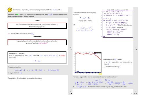
Numerical experiment with nearly singular
Code 2.5.4: small residuals for GE
1 n = 10; u = ( 1 : n ) ’ / 3 ; v =
( 1 . / u ) .∗( −1) . ^ ( ( 1 : n ) ’ ) ;
matrix
2 x = ones ( 1 0 ,1) ; nx = norm( x , ’ i n f ’ ) ;
A = uv T 3
+ ǫI ,
4 r e s u l t = [ ] ;
singular rank-1 matrix
5 for e p s i l o n = 10.^(−5:−0.5:−14)
6 A = u∗v ’ + e p s i l o n∗eye ( n ) ;
with
7 b = A∗x ; nb = norm( b , ’ i n f ’ ) ;
8 x t = A \ b ; % Gaussian elimination
norm( r , ’ i n f ’ ) / nb ,
cond (A, ’ i n f ’ ) ] ;
11 end
In practice Gaussian elimination/LU-factorization with partial pivoting
produces “relatively small residuals”
Ôº½¾ ¾º
Ôº½¾ ¾º
Definition 2.5.8 (Residual).
Given an approximate solution ˜x ∈ K n of the LSE Ax = b (A ∈ K n,n , b ∈ K n ), its residual
is the vector
r = b − A˜x .
10 2
10 0
10 −2
10 −4
10 −6
10 −8
ε
relative error
relative residual
Observations (w.r.t ‖·‖ ∞ -norm)
for ǫ ≪ 1 large relative error in computed solution
˜x
Simple consideration:
10 −10
10 −12
small residuals for any ǫ
(A + ∆A)˜x = b ⇒ r = b − A˜x = ∆A˜x ⇒ ‖r‖ ≤ ‖∆A‖ ‖˜x‖ ,
10 −14
for any vector norm ‖·‖.
Example 2.5.3 (Small residuals by Gaussian elimination).
Ôº½¾ ¾º
10 −16
10 −14 10 −13 10 −12 10 −11 10 −10 10 −9 10 −8 10 −7 10 −6 10 −5
Fig. 34
How can a large relative error be reconciled with a small relative residual ?
Ax = b ↔ A˜x ≈ b
{ ∥
A(x − ˜x) = r ⇒ ‖x − ˜x‖ ≤ A −1∥ ∥ ‖r‖ ‖x − ˜x‖
∥
⇒ ≤ ‖A‖ ∥A −1∥ ∥ ‖r‖
Ax = b ⇒ ‖b‖ ≤ ‖A‖ ‖x‖
‖x‖
‖b‖ . (2.5.6)
➣ If ‖A‖ ∥ ∥A −1∥ ∥ ≫ 1, then a small relative residual may not imply a small relative error.
Ôº½¾ ¾º
✸