Numerical Methods Contents - SAM

➤ Linear system of equations with tridiagonal s.p.d. (→ Def. 2.7.1, Lemma 2.7.4) coefficient
matrix → c 0 , ...,c n
Thm. 2.6.6 ⇒ computational effort for the solution = O(n)
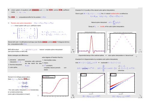
Example 9.4.3 (Locality of the natural cubic spline interpolation).
Given a grid M := {t 0 < t 1 < · · · < t n } the ith natural cardinal spline is defined as
L i ∈ S 3,M , L i (t j ) = δ ij , L ′′
i (t 0) = L ′′
i (t n) = 0 .
➂ Periodic cubic spline interpolation: s ′ (t 0 ) = s ′ (t n ), s ′′ (t 0 ) = s ′′ (t n )
n × n-linear system with s.p.d. coefficient matrix
⎛
⎞
a 1 b 1 0 · · · 0 b 0
b 1 a 2 b 2 0
A :=
0 . . . ... . .. .
⎜ . ... . .. ... 0
,
⎝ 0 .
⎟
.. a n−1 b n−1 ⎠
b 0 0 · · · 0 b n−1 a 0
b i := 1
h i+1
, i = 0, 1, ...,n − 1 ,
a i := 2 h i
+ 2
h i+1
, i = 0, 1, . ..,n − 1 .
Solved with rank-1-modifications technique (see Section 2.9.0.1, Lemma 2.9.1) + tridiagonal elimination,
computational effort O(n)
MATLAB-function: v = spline(t,y,x): natural / complete spline interpolation
(see spline-toolbox in MATLAB)
Ôº¾ º
1.2
1
0.8
0.6
0.4
0.2
0
n∑
Natural spline interpolant: s(t) = y j L j (t) .
j=0
Decay of L i ↔ locality of the cubic spline interpolation.
Cardinal cubic spline function
Cardinal cubic spline in middle points of the intervals
10 0
10 −1
Value of the cardinal cubic splines
10 −2
10 −3
10 −4
Ôº¿½ º
−5
Notice analogies and differences:
extra degrees of freedom fixed by:
1. piecewise polynomial
1. intermediate nodes,
interpolant, d = 3,
piecewise cubic polynomials
that match the data 2. slopes,
2. Hermite interpolant,
(t i , y i )
3. C 2 -constraint,
3. cubic spline,
complete/natural/periodic
constraint.
Exponential decay of the cardinal splines ➞ cubic spline interpolation is “almost local”
✸
Example 9.4.4 (Approximation by complete cubic spline interpolants).
Grid M := {−1 + n 2j}n j=0 , n ∈ N ➙ meshwidth h = 2/n, I = [−1, 1]
⎧
1
⎪⎨ 0 , if t < −
f 1 (t) =
1 + e −2t ∈ 5 2 ,
C∞ (I) , f 2 (t) = 1
2 ⎪⎩
(1 + cos(π(t − 3 5 ))) , if − 2 5 < t < 5 3 , ∈ C 1 (I) .
1 otherwise.
Remark 9.4.2 (Shape preservation).
Data s(t j ) = y j from Ex. 9.1.1 and
c 0 := y 1 − y 0
t 1 − t 0
,
c n := y n − y n−1
t n − t n−1
.
The cubic spline interpolant is not monotonicityor
curvature-preserving
(cubic spline interpolation is linear!)
△
s(t)
1.2
1
0.8
0.6
0.4
0.2
0
Data points
Cubic spline interpolant
−0.2
−1 −0.8 −0.6 −0.4 −0.2 0 0.2 0.4 0.6 0.8 1
t
Ôº¿¼ º
||s−f||
L ∞ −Norm
L 2 −Norm
10 −4
10 −6
10 −8
10 −10
10 −12
10 −2 10 −1 10 0
10 −2 Meshwidth h
‖f 1 − s‖ L ∞ ([−1,1]) = O(h4 )
||s−f||
L ∞ −Norm
10 −1 L 2 −Norm
10 −2
10 −3
10 −4
10 −5
10 −6
10 −7
10 −2 10 −1 10 0
10 0 Meshwidth h
‖f 2 − s‖ L ∞ ([−1,1]) = O(h2 )
Ôº¿¾ º