Numerical Methods Contents - SAM

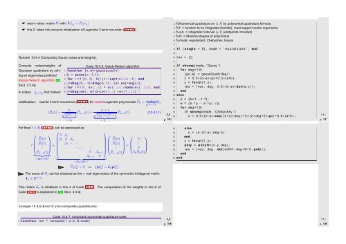
☛ return value: matrix V with (V) ij = P i (x j )
☛ line 2: takes into account initialization of Legendre 3-term recursion (10.4.10)
Remark 10.4.4 (Computing Gauss nodes and weights).
Compute nodes/weights of
Gaussian quadrature by solving
an eigenvalue problem!
(Golub-Welsch algorithm [16,
Sect. 3.5.4])
In codes:
ξ j , ω j from tables!
Code 10.4.5: Golub-Welsch algorithm
1 function [ x ,w]= gaussquad ( n )
2 b = zeros ( n−1,1) ;
3 for i = 1 : ( n−1) , b ( i ) = i / sqrt (4∗ i ∗ i −1) ; end
4 J=diag ( b,−1)+diag ( b , 1 ) ; [ ev , ew]= eig ( J ) ;
5 for i =1:n , ev ( : , i ) = ev ( : , i ) . / norm( ev ( : , i ) ) ; end
6 x=diag (ew) ; w=(2∗( ev ( 1 , : ) .∗ ev ( 1 , : ) ) ) ’ ;
Justification: rewrite 3-term recurrence (10.4.10) for scaled Legendre polynomials ˜P n = 1 √ n+1/2
P n
t ˜P n
n + 1
n (t) = √
} 4n {{ 2 ˜Pn−1 (t) + √
− 1}
4(n + 1) 2 − 1
} {{ }
=:β n
△
2 % Numerical quadrature on [a,b] by polynomial quadrature formula
3 % f -> function to be integrated (handle), must support vector arguments
4 % a,b -> integration interval [a,b] (endpoints included)
5 % N -> Maximal degree of polynomial
6 % mode: equidistant, Chebychev, Gauss
7
8 i f ( nargin < 5) , mode = ’ e q u i d i s t a n t ’ ; end
9
10 res = [ ] ;
11
12 i f strcmp (mode , ’ Gauss ’ )
13 for deg=1:N
14 [ gx ,w] = gaussQuad ( deg ) ;
15 x = 0.5∗( b−a ) ∗gx +0.5∗(a+b ) ;
16 y = feval ( f , x ) ;
17 res = [ res ; deg , 0.5∗( b−a ) ∗dot (w, y ) ] ;
18 end
19 else
20 p = (N+1: −1:1) ;
21 w = ( b . ^ p − a . ^ p ) . / p ;
22 for deg=1:N
23 i f strcmp (mode , ’ Chebychev ’ )
Ôº¼ ½¼º
Ôº¼ ½¼º
˜Pn+1 (t) . (10.4.11)
24 x = 0.5∗(b−a ) ∗cos ( ( 2 ∗ ( 0 : deg ) +1) / ( 2∗ deg+2)∗pi ) +0.5∗(a+b ) ;
=:β n+1
For fixed t ∈ R (10.4.11) can be expressed as
⎛
⎞
⎛ ⎞ 0 β 1
⎛ ⎞ ⎛ ⎞
˜P 0 (t)
β 1 0 β 2
˜P ˜P
t ⎜ 1 (t)
⎟ =
β . 2
.. . ..
0 (t)
˜P
⎝ . ⎠
.
⎜
.. ... ...
⎜ 1 (t)
⎟
⎟ ⎝ . ⎠ + ⎜
0.
⎟
⎝ 0 ⎠
˜P n−1 (t) ⎝
0 β n−1 ⎠ ˜P n−1 (t) β n ˜Pn (t)
} {{ }
β n−1 0
=:p(t)∈R n } {{ }
=:J n ∈R n,n
˜P n (ξ) = 0 ⇔ ξp(ξ) = J n p(ξ) .
25 else
26 x = ( a : ( b−a ) / deg : b ) ;
27 end
28 y = feval ( f , x ) ;
29 poly = p o l y f i t ( x , y , deg ) ;
30 res = [ res ; deg , dot (w(N+1−deg :N+1) , poly ) ] ;
31 end
32 end
The zeros of P n can be obtained as the n real eigenvalues of the symmetric tridiagonal matrix
J n ∈ R n,n !
This matrix J n is initialized in line 4 of Code 10.4.4. The computation of the weights in line 6 of
Code 10.4.4 is explained in [16, Sect. 3.5.4].
△
Example 10.4.6 (Error of (non-composite) quadratures).
Ôº¼ ½¼º
Code 10.4.7: important polynomial quadrature rules
1 function res = numquad( f , a , b ,N, mode)
Ôº¼ ½¼º