Numerical Methods Contents - SAM

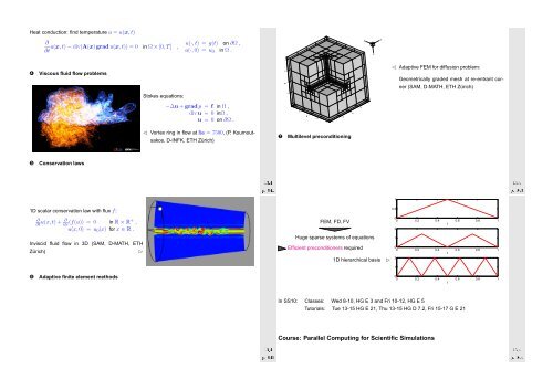
Z
Heat conduction: find temperature u = u(x, t)
∂
∂t u(x, t) − div(A(x)grad u(x, t)) = 0 in Ω × [0, T] , u(·, t) = g(t) on ∂Ω ,
u(·, 0) = u 0 in Ω .
X
Z
Y
­1
➍
Viscous fluid flow problems
­0.5
0
✁ Adaptive FEM for diffusion problem:
Geometrically graded mesh at re-entrant corner
(SAM, D-MATH, ETH Zürich)
Stokes equations:
0.5
−∆u + gradp = f in Ω ,
divu = 0 inΩ ,
u = 0 on ∂Ω .
1
1
0.5
X
0
­0.5
­1
­1
­0.5
0
Y
0.5
1
✁ Vortex ring in flow at Re = 7500, (P. Koumoutsakos,
D-INFK, ETH Zürich)
➐
Multilevel preconditioning
➎
Conservation laws
Ôº½ ½¿º
Ôº¿ ½¿º
1
1D scalar conservation law with flux f:
∂
∂t u(x,t) + ∂x ∂ (f(u)) = 0 in R × R+ ,
u(x, 0) = u 0 (x) for x ∈ R .
Inviscid fluid flow in 3D (SAM, D-MATH, ETH
Zürich)
✄
FEM, FD, FV
Huge sparse systems of equations
Efficient preconditioners required
1D hierarchical basis
✄
0.5
0
0 0.2 0.4 0.6 0.8 1
t
2
1
0
0 0.2 0.4 0.6 0.8 1
t
2
1
➏
Adaptive finite element methods
0
0 0.2 0.4 0.6 0.8 1
t
In SS10: Classes: Wed 8-10, HG E 3 and Fri 10-12, HG E 5
Tutorials: Tue 13-15 HG E 21, Thu 13-15 HG D 7.2, Fri 15-17 G E 21
Ôº¾ ½¿º
Course: Parallel Computing for Scientific Simulations
Ôº ½¿º