Numerical Methods Contents - SAM

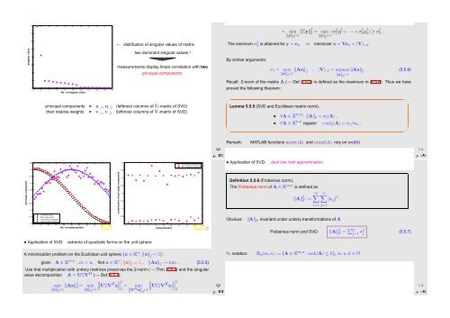
0 2 4 6 8 10 12 14 16 18 20
singular value
16
14
12
10
8
6
4
2
0
No. of singular value
← distribution of singular values of matrix
two dominant singular values !
measurements display linear correlation with two
principal components
= min
‖y‖ 2 =1 ‖Σy‖2 2 = min ‖y‖ 2 =1 (σ2 1 y2 1 + · · · + σ2 ny 2 n) ≥ σ 2 n .
The minimum σ 2 n is attained for y = e n ⇒ minimizer x = Ve n = (V) :,n .
By similar arguments:
σ 1 = max
‖x‖ 2 =1 ‖Ax‖ 2
, (V) :,1 = argmax ‖Ax‖ 2 . (5.5.6)
‖x‖ 2 =1
Recall: 2-norm of the matrix A (→ Def. 2.5.2) is defined as the maximum in (5.5.6). Thus we have
proved the following theorem:
✬
✩
principal components = u·,1 , u·,2 (leftmost columns of U-matrix of SVD)
their relative weights = v·,1 , v·,2 (leftmost columns of V-matrix of SVD)
Lemma 5.5.5 (SVD and Euclidean matrix norm).
• ∀A ∈ K m,n : ‖A‖ 2 = σ 1 (A) ,
• ∀A ∈ K n,n regular: cond 2 (A) = σ 1 /σ n .
Ôº¿ º
✫
Remark:
MATLAB functions norm(A) and cond(A) rely on svd(A)
✪
Ôº º
0.25
0.4
1st principal component
2nd principal component
• Application of SVD:
best low rank approximation
0.2
0.35
principal component
0.15
0.1
0.05
0
−0.05
−0.1
−0.15
1st model vector
2nd model vector
1st principal component
2nd principal component
−0.2
20 25 30
No. of measurement
45 50
Fig. 86
0 5 10 15 35 40
contribution of principal component
0.3
0.25
0.2
0.15
0.1
0.05
0
0 2 4 6 8 10 12 14 16 18 20
measurement
Fig. 87 ✸
Definition 5.5.6 (Frobenius norm).
The Frobenius norm of A ∈ K m,n is defined as
Obvious:
‖A‖ 2 F := m ∑
i=1 j=1
n∑
|a ij | 2 .
‖A‖ F invariant under unitary transformations of A
Frobenius norm and SVD:
‖A‖ 2 F = ∑ p
j=1 σ2 j (5.5.7)
• Application of SVD:
extrema of quadratic forms on the unit sphere
A minimization problem on the Euclidean unit sphere {x ∈ K n : ‖x‖ 2 = 1}:
✎ notation:
R k (m, n) := {A ∈ K m,n : rank(A) ≤ k}, m, n,k ∈ N
given A ∈ K m,n , m > n, find x ∈ K n , ‖x‖ 2 = 1 , ‖Ax‖ 2 → min . (5.5.5)
Use that multiplication with unitary matrices preserves the 2-norm (→ Thm. 2.8.2) and the singular
value decomposition A = UΣV H (→ Def. 5.5.2):
min
‖x‖ 2 =1 ‖Ax‖2 2 = min ∥
∥UΣV H x∥ 2 = min ∥
∥UΣ(V H x) ∥ 2
‖x‖ 2 =1
2 ‖V H x‖ 2 =1
2
Ôº º
Ôº º