Numerical Methods Contents - SAM

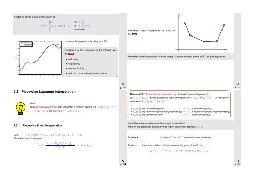
created by taking points on the graph of
⎧
⎪⎨ 0 if t < −5 2 ,
f(t) = 1
2 ⎪⎩
(1 + cos(π(t − 5 3))) if − 5 2 < t < 3 5 ,
1 otherwise.
Piecewise linear interpolant of data in
Fig. 104:
y
1.2
1
Polynomial
Measure pts.
Natural f
← Interpolating polynomial, degree = 10
y
0.8
0.6
0.4
0.2
0
−0.2
−0.4
−0.6
−1 −0.8 −0.6 −0.4 −0.2 0 0.2 0.4 0.6 0.8 1
t
Oscillations at the endpoints of the interval (see
Ex. 8.4.3)
• No locality
• No positivity
• No monotonicity
9.2 Piecewise Lagrange interpolation
Idea:
• No local conservation of the curvature
use piecewise polynomials with respect to a partition (mesh) M := {a = x 0 < x 1 <
. .. < x m = b} of the interval I := [a,b], a < b.
✸
Ôº¿ º¾
Piecewise linear interpolation means simply “connect the data points in R 2 using straight lines”.
✬
Theorem 9.2.1 (Local shape preservation by piecewise linear interpolation).
Let s ∈ C([t 0 , t n ]) be the piecewise linear interpolant of (t i ,y i ) ∈ R 2 , i = 0, ...,n, for every
subinterval I = [t j ,t k ] ⊂ [t 0 ,t n ]:
if (t i , y i )| I are positive/negative
⇒ s| I is positive/negative,
if (t i , y i )| I are monotonic (increasing/decreasing) ⇒ s| I is monotonic (increasing/decreasing),
if (t i , y i )| I are convex/concave
⇒ s| I is convex/concave.
t
✩
Ôº º¾
✫
✪
9.2.1 Piecewise linear interpolation
Local shape preservation = perfect shape preservation!
None of this properties carries over to higher polynomial degrees d > 1.
Data: (t i ,y i ) ∈ R 2 , i = 0,...,n, n ∈ N, t 0 < t 1 < · · · < t n .
Piecewise linear interpolant:
Drawback:
f is only C 0 but not C 1 (no continuous derivative).
s(x) = (t i+1 − t)y i + (t − t i )y i+1
t i+1 − t i
t ∈ [t i ,t i+1 ].
Ôº º¾
Obvious:
linear interpolation is linear (as mapping y ↦→ s) and local:
y j = δ ij , i, j = 0,...,n ⇒ supp(s) ⊂ [t i−1 ,t i+1 ] .
Ôº º¾