Numerical Methods Contents - SAM

Non-linear system of equations from nodal analysis (→ Ex. 2.0.1):
➀ : R 3 (U 1 − U + ) + R 1 (U 1 − U 3 ) + I B (U 5 − U 1 , U 5 − U 2 ) = 0 ,
➁ : R e U 2 + I E (U 5 − U 1 , U 5 − U 2 ) + I E (U 3 − U 4 , U 3 − U 2 ) = 0 ,
➂ : R 1 (U 3 − U 1 ) + I B (U 3 − U 4 , U 3 − U 2 ) = 0 ,
➃ : R 4 (U 4 − U + ) + I C (U 3 − U 4 , U 3 − U 2 ) = 0 ,
➄ : R b (U 5 − U in ) + I B (U 5 − U 1 , U 5 − U 2 ) = 0 .
5 equations ↔ 5 unknowns U 1 ,U 2 ,U 3 ,U 4 ,U 5
(3.0.2)
✬
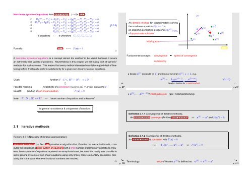
An iterative method for (approximately) solving
the non-linear equation F(x) = 0 is
an algorithm generating a sequence (x (k) ) k∈N0
of approximate solutions.
✫
Initial guess
✩
✪
D
x (2) x (3)
Φ
x ∗
x (1) x (4)
x (6)
x (0) x (5)
Formally: (3.0.2) ←→ F(u) = 0
✸
Fig. 28
A non-linear system of equations is a concept almost too abstract to be useful, because it covers
an extremely wide variety of problems . Nevertheless in this chapter we will mainly look at “generic”
methods for such systems. This means that every method discussed may take a good deal of finetuning
before it will really perform satisfactorily for a given non-linear system of equations.
Fundamental concepts: convergence ➡ speed of convergence
consistency
Ôº¾¿ ¿º¼
Possible meaning: Availability of a procedure function y=F(x) evaluating F
Given: function F : D ⊂ R n ↦→ R n , n ∈ N
⇕
• iterate x (k) depends on F and (one or several) x (n) , n < k, e.g.,
x (k) = Φ F (x (k−1) , ...,x (k−m) )
} {{ }
iteration function for m-point method
(3.1.1)
Ôº¾¿ ¿º½
Sought: solution of non-linear equation F(x) = 0
Note: F : D ⊂ R n ↦→ R n ↔ “same number of equations and unknowns”
• x (0) ,...,x (m−1) = initial guess(es)
(ger.: Anfangsnäherung)
In general no existence & uniqueness of solutions
Definition 3.1.1 (Convergence of iterative methods).
An iterative method converges (for fixed initial guess(es)) :⇔ x (k) → x ∗ and F(x ∗ ) = 0.
3.1 Iterative methods
Remark 3.1.1 (Necessity of iterative approximation).
Gaussian elimination (→ Sect. 2.1) provides an algorithm that, if carried out in exact arithmetic, computes
the solution of a linear system of equations with a finite number of elementary operations. However,
linear systems of equations represent an exceptional case, because it is hardly ever possible to
solve general systems of non-linear equations using only finitely many elementary operations. Certainly
this is the case whenever irrational numbers are involved.
△
Ôº¾¿ ¿º½
Definition 3.1.2 (Consistency of iterative methods).
An iterative method is consistent with F(x) = 0
:⇔ Φ F (x ∗ , . ..,x ∗ ) = x ∗ ⇔ F(x ∗ ) = 0
Ôº¾¼ ¿º½
Terminology: error of iterates x (k) is defined as: e (k) := x (k) − x ∗