Numerical Methods Contents - SAM

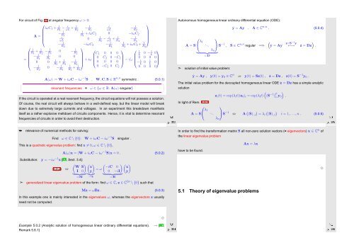
For circuit of Fig. 55 at angular frequency ω > 0:
⎛
iωC 1 + R 1 − 1 ωL i + R 1 − 1 i
2 R 1 ωL − 1 ⎞
R 2
−
A =
1 1 R 1 R1
+ iωC 2 0 −iωC 2
⎜ i
⎝ ωL 0 1
R5
− ωL i + R 1 − 1 ⎟
4 R 4 ⎠
−R 1 −iωC 2 2 −R 1 1
4 R2
+ iωC 2 + R 1 ⎛
4
1
R + 1 R 1 − 2 R 1 0 − 1 ⎞
⎛
⎞ ⎛
1 R 1
2
−
=
R 1 1 C 1 0 0 0 L
1 R1
0 0
⎜
⎝ 0 0 1
R5
+ R 1 − 1 ⎟
4 R 4 ⎠ + iω ⎜ 0 C 2 0 −C 2
⎟
⎝ 0 0 0 0 ⎠ − 0 − L 1 0
⎞
i/ω ⎜ 0 0 0 0
⎝− −R 1 0 − 1 1
2 R 4 R2
+ R 1 L 1 0 ⎟
1
L 0⎠
0 −C 2 0 C 2 0 0 0 0
4
✗
✖
A(ω) := W + iωC − iω −1 S , W,C,S ∈ R n,n symmetric . (5.0.1)
resonant frequencies = ω ∈ {ω ∈ R: A(ω) singular}
If the circuit is operated at a real resonant frequency, the circuit equations will not possess a solution.
Of course, the real circuit will always behave in a well-defined way, but the linear model will break
down due to extremely large currents and voltages.
In an experiment this breakdown manifests
itself as a rather explosive meltdown of circuits components. Hence, it is vital to determine resonant
frequencies of circuits in order to avoid their destruction.
✔
✕
Ôº¿¿ º¼
Autonomous homogeneous linear ordinary differential equation (ODE):
➣
⎛
A = S⎝ λ ⎞
1 . .. ⎠S −1 , S ∈ C n,n regular =⇒
λ n
} {{ }
=:D
solution of initial value problem:
ẏ = Ay , A ∈ C n,n . (5.0.4)
(
ẏ = Ay z=S−1 y
←→
)
ż = Dz .
ẏ = Ay , y(0) = y 0 ∈ C n ⇒ y(t) = Sz(t) , ż = Dz , z(0) = S −1 y 0 .
The initial value problem for the decoupled homogeneous linear ODE ż = Dz has a simple analytic
solution
In light of Rem. 1.2.1:
⎛
A = S⎝ λ 1 . . .
( )
z i (t) = exp(λ i t)(z 0 ) i = exp(λ i t) (S −1 ) T i,: y 0 .
⎞
⎠S −1 ⇔ A ( ) ( )
(S) :,i = λi (S):,i
λ n
Ôº¿ º¼
i = 1, ...,n . (5.0.5)
➥
relevance of numerical methods for solving:
Find ω ∈ C \ {0}: W + iωC − iω −1 S singular .
This is a quadratic eigenvalue problem: find x ≠ 0, ω ∈ C \ {0},
Substitution: y = −iω −1 x [41, Sect. 3.4]:
( )( W S x
(5.0.2) ⇔
I 0 y)
} {{ }}{{}
:=M :=z
➣
A(ω)x = (W + iωC − iω −1 S)x = 0 . (5.0.2)
(
−iC 0
= ω
0 −iI
} {{ }
:=B
)( x
y)
generalized linear eigenvalue problem of the form: find ω ∈ C, z ∈ C 2n \ {0} such that
Mz = ωBz . (5.0.3)
In this example one is mainly interested in the eigenvalues ω, whereas the eigenvectors z usually
need not be computed.
In order to find the transformation matrix S all non-zero solution vectors (= eigenvectors) x ∈ C n of
the linear eigenvalue problem
Ax = λx
have to be found.
✸
5.1 Theory of eigenvalue problems
Example 5.0.2 (Analytic solution of homogeneous linear ordinary differential equations). → [40,
Remark 5.6.1]
✸
Ôº¿ º¼
Ôº¿ º½