Numerical Methods Contents - SAM

However, it would be foolish not to use the better value y k+1 = ˜Ψ hk y k , since it is available for
free. This is what is done in every implementation of adaptive methods, also in Code 11.5.2, and this
choice can be justified by control theoretic arguments [12, Sect. 5.2].
Example 11.5.4 (Simple adaptive stepsize control).
IVP for ODE
ẏ = cos(αy) 2 , α > 0, solution y(t) = arctan(α(t −c))/α for y(0) ∈] −π/2,π/2[
Simple adaptive timestepping based on explicit Euler (11.2.1) and explicit trapezoidal rule (11.4.3)
Code 11.5.5: MATLAB function for Ex. 11.5.4
1 function o d e i n t a d a p t d r i v e r ( T , a , r e l t o l , a b s t o l )
2 % Simple adaptive timestepping strategy of Code 11.5.2
3 % based on explicit Euler (11.2.1) and explicit trapezoidal
4 % rule (11.4.3)
5
Ôº½ ½½º
10 i f ( nargin < 1) , T = 2 ; end
6 % Default arguments
7 i f ( nargin < 4) , a b s t o l = 1E−4; end
8 i f ( nargin < 3) , r e l t o l = 1E−2; end
9 i f ( nargin < 2) , a = 20; end
%f ’ , r e l t o l , abstol , a ) ) ;
33 xlabel ( ’ { \ b f t } ’ , ’ f o n t s i z e ’ ,14) ;
34 ylabel ( ’ { \ b f y } ’ , ’ f o n t s i z e ’ ,14) ;
35 legend ( ’ y ( t ) ’ , ’ y_k ’ , ’ r e j e c t i o n ’ , ’ l o c a t i o n ’ , ’ northwest ’ ) ;
36 p r i n t −depsc2 ’ . . / PICTURES/ o d e i n tadaptsol . eps ’ ;
37
38 f p r i n t f ( ’%d timesteps , %d r e j e c t e d
timesteps \ n ’ , length ( t ) −1,length ( r e j ) ) ;
39
40 % Plotting estimated and true errors
41 figure ( ’name ’ , ’ ( estimated ) e r r o r ’ ) ;
42 plot ( t , abs ( s o l ( t ) − y ) , ’ r + ’ , t , ee , ’m∗ ’ ) ;
43 xlabel ( ’ { \ b f t } ’ , ’ f o n t s i z e ’ ,14) ;
44 ylabel ( ’ { \ b f e r r o r } ’ , ’ f o n t s i z e ’ ,14) ;
45 legend ( ’ t r u e e r r o r | y ( t_k )−y_k | ’ , ’ estimated e r r o r
EST_k ’ , ’ l o c a t i o n ’ , ’ northwest ’ ) ;
46 t i t l e ( s p r i n t f ( ’ Adaptive timestepping , r t o l = %f , a t o l = %f , a =
%f ’ , r e l t o l , abstol , a ) ) ;
47 p r i n t −depsc2 ’ . . / PICTURES/ o d e i n t a d a p t e r r . eps ’ ;
Ôº¿ ½½º
11
12 % autonomous ODE ẏ = cos(ay) and its general solution
13 f = @( y ) ( cos ( a∗y ) . ^ 2 ) ; s o l = @( t ) ( atan ( a∗( t −1) ) / a ) ;
14 % Initial state y 0
15 y0 = s o l ( 0 ) ;
16
17 % Discrete evolution operators, see Def. 11.2.1
18 Psilow = @( h , y ) ( y + h∗ f ( y ) ) ; % Explicit Euler (11.2.1)
19 % Explicit trapzoidal rule (11.4.3)
20 Psihigh = @( h , y ) ( y + 0.5∗h∗( f ( y ) + f ( y+h∗ f ( y ) ) ) ) ;
21
22 % Heuristic choice of initial timestep and h min
23 h0 = T /(100∗(norm( f ( y0 ) ) +0.1) ) ; hmin = h0 /10000;
24 % Main adaptive timestepping loop, see Code 11.5.2
25 [ t , y , r e j , ee ] =
odeintadapt_ext ( Psilow , Psihigh , T , y0 , h0 , r e l t o l , abstol , hmin ) ;
26
y
0.08
0.06
0.04
0.02
0
−0.02
−0.04
−0.06
y(t)
y k
rejection
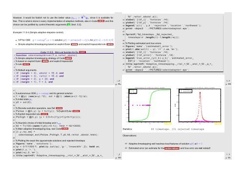
Adaptive timestepping, rtol = 0.010000, atol = 0.000100, a = 20.000000
−0.08
0 0.2 0.4 0.6 0.8 1 1.2 1.4 1.6 1.8 2
t
Statistics:
Observations:
Fig. 148
error
0.025
0.02
0.015
0.01
0.005
Adaptive timestepping, rtol = 0.010000, atol = 0.000100, a = 20.000000
true error |y(t k
)−y k
|
estimated error EST k
Fig. 149
0
0 0.2 0.4 0.6 0.8 1 1.2 1.4 1.6 1.8 2
t
66 timesteps, 131 rejected timesteps
27 % Plotting the exact the approximate solutions and rejected timesteps
28 figure ( ’name ’ , ’ s o l u t i o n s ’ ) ;
29 tp = 0 :T/1000:T ; plot ( tp , s o l ( tp ) , ’ g−’ , ’ l i n e w i d t h ’ ,2) ; hold on ;
Ôº¾ ½½º
30 plot ( t , y , ’ r . ’ ) ;
31 plot ( r e j , 0 , ’m+ ’ ) ;
32 t i t l e ( s p r i n t f ( ’ Adaptive timestepping , r t o l = %f , a t o l = %f , a =
☞ Adaptive timestepping well resolves local features of solution y(t) at t = 1
☞ Estimated error (an estimate for the one-step error) and true error are not related!
Ôº ½½º