Numerical Methods Contents - SAM

Evident: symmetry of à − bbT
a 11
∈ R n−1,n−1
As A s.p.d. (→ Def. 2.7.1), for every y ∈ R n−1 \ {0}
( ) T (a11
0 <
− bT y b T ) ( )
a − bT y
11
y b Ã
a 11
y
à − bbT
a 11
positive definite.
The proof can also be based on the identities
( )
(A)1:n−1,1:n−1 (A) 1:n−1,n
=
(A) n,1:n−1 (A) n,n
= y T (Ã − bbT
a 11
)y .
( L1 0
l T 1
✷
)( )
U1 u
, (2.6.4)
0 γ
⇒ (A) 1:n−1,1:n−1 = L 1 U 1 , L 1 u = (A) 1:n−1,n , U T 1 l = (A)T n,1:n−1 , lT u + γ = (A) n,n ,
noticing that the principal minor (A) 1:n−1,1:n−1 is also s.p.d. This allows a simple induction argument.
Note: no pivoting required (→ Sect. 2.3)
(partial pivoting always picks current pivot row)
Ôº½ ¾º
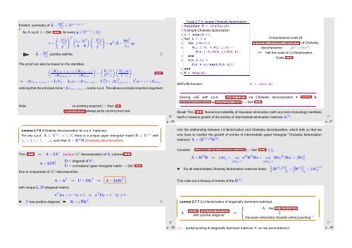
Code 2.7.3: simple Cholesky factorization
1 function R = c h o l f a c (A)
2 % simple Cholesky factorization
3 n = size (A, 1 ) ;
4 for k = 1 : n
5 for j =k +1:n
6 A( j , j : n ) = A( j , j : n ) −
A( k , j : n ) ∗A( k , j ) /A( k , k ) ;
7 end
8 A( k , k : n ) =
A( k , k : n ) / sqrt (A( k , k ) ) ;
9 end
10 R = t r i u (A) ;
MATLAB function:
★
✧
Computational costs (#
elementary arithmetic operations) of Cholesky
decomposition:
1
6 n3 + O(n 2 )
(➣ half the costs of LU-factorization,
R = chol(A)
Code. 2.2.1)
Solving LSE with s.p.d. system matrix via Cholesky decomposition + forward &
backward substitution is numerically stable (→ Def. 2.5.5)
Recall Thm. 2.5.7: Numerical instability of Gaussian elimination (with any kind of pivoting) manifests
itself in massive growth of the entries of intermediate elimination matrices A (k) .
✥
✦
Ôº½ ¾º
✬
Lemma 2.7.6 (Cholesky decomposition for s.p.d. matrices).
For any s.p.d. A ∈ K n,n , n ∈ N, there is a unique upper triangular matrix R ∈ K n,n with
r ii > 0, i = 1, ...,n, such that A = R H R (Cholesky decomposition).
✫
Thm. 2.7.5 ⇒ A = LU (unique LU-decomposition of A, Lemma 2.2.3)
A = LDŨ , D ˆ= diagonal of U ,
Ũ ˆ= normalized upper triangular matrix → Def. 2.2.1
Due to uniqueness of LU-decomposition
with unique L, D (diagonal matrix)
A = A T ⇒ U = DL T ⇒ A = LDL T ,
✩
✪
Use the relationship between LU-factorization and Cholesky decomposition, which tells us that we
only have to monitor the growth of entries of intermediate upper triangular “Cholesky factorization
matrices” A = (R (k) ) H R (k) .
Consider: Euclidean vector norm/matrix norm (→ Def. 2.5.2) ‖·‖ 2
➤
A = R H R ⇒ ‖A‖ 2 = sup x H R H Rx = sup (Rx) H (Rx) = ‖R‖ 2 2 .
‖x‖ 2 =1
‖x‖ 2 =1
∥
For all intermediate Cholesky factorization matrices holds: ∥(R (k) ) H∥ ∥ ∥ ∥2 = ∥R (k)∥ ∥ ∥2 = ‖A‖ 1/2
2
This rules out a blowup of entries of the R (k) .
x T Ax > 0 ∀x ≠ 0 ⇒ y T Dy > 0 ∀y ≠ 0 .
➤ D has positive diagonal ➨ R = √ DL T . ✷
Ôº½ ¾º
✬
Lemma 2.7.7 (LU-factorization of diagonally dominant matrices).
⎧
⎨
A has LU-factorization
regular, diagonally dominant
A ⇔
⇕
with positive diagonal ⎩
Gaussian elimination feasible without pivoting (∗)
Ôº½ ¾º
✫
✪
(∗): partial pivoting & diagonally dominant matrices ➣ no row permutations !
✩