Numerical Methods Contents - SAM

✎ Notation (Newton): dot ˙ ˆ= (total) derivative with respect to time t
y ˆ= population density, [y] = 1 m 2
Part III
growth rate α − βy with growth coefficients α, β > 0, [α] = 1 m2
s , [β] = s : decreases due to
more fierce competition as population density increases.
Note:
we can only compute a solution of (11.1.1), when provided with an initial value y(0).
Integration of Ordinary Differential Equations
Ôº¾½ ½¼º
Ôº¾¿ ½½º½
11 Single Step Methods
11.1 Initial value problems (IVP) for ODEs
y
1.5
1
0.5
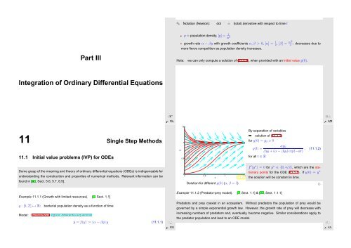
By separation of variables
➥ solution of (11.1.1)
for y(0) = y 0 > 0
y(t) =
for all t ∈ R
αy 0
βy 0 + (α − βy 0 ) exp(−αt) , (11.1.2)
Some grasp of the meaning and theory of ordinary differential equations (ODEs) is indispensable for
understanding the construction and properties of numerical methods. Relevant information can be
found in [40, Sect. 5.6, 5.7, 6.5].
0
0 0.5 1 1.5
t
Fig. 122
Solution for different y(0) (α,β = 5)
f ′ (y ∗ ) = 0 for y ∗ ∈ {0, α/β}, which are the stationary
points for the ODE (11.1.1). If y(0) = y ∗
the solution will be constant in time.
✸
Example 11.1.1 (Growth with limited resources). [1, Sect. 1.1]
y : [0, T] ↦→ R:
Model:
Ôº¾¾ ½½º½
autonomous logistic differential equations
ẏ = f(y) := (α − βy) y (11.1.1)
bacterial population density as a function of time
Example 11.1.2 (Predator-prey model). [1, Sect. 1.1] & [21, Sect. 1.1.1]
Predators and prey coexist in an ecosystem.
Without predators the population of prey would be
governed by a simple exponential growth law. However, the growth rate of prey will decrease with
increasing numbers of predators and, eventually, become negative. Similar considerations apply to
the predator population and lead to an ODE model.
Ôº¾ ½½º½