Numerical Methods Contents - SAM

1.2
equality in (8.2.10) for y := (sgn(L j (t ∗ ))) n j=0 , t∗ := argmax t∈I
∑ ni=0
|L i (t)|.
✷
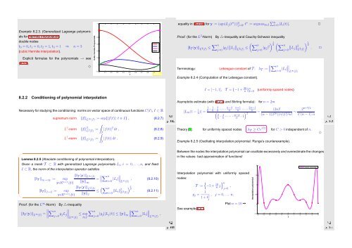
Example 8.2.3. (Generalized Lagrange polynomials
for Hermite Interpolation)
double nodes
t 0 = 0, t 1 = 0, t 2 = 1, t 3 = 1 ⇒ n = 3
(cubic Hermite interpolation).
Explicit formulas for the polynomials → see
(9.3.2).
✸
Cubic Hermite Polynomials
1
0.8
0.6
0.4
0.2
0
−0.2
0 0.1 0.2 0.3 0.4 0.5 0.6 0.7 0.8 0.9 1
t
p 0
p 1
p 2
p 3
Fig. 99
Proof. (for the L 2 -Norm)
By △-inequality and Cauchy-Schwarz inequality
‖I T (y)‖ L 2 (I) ≤ ∑ n
j=0 |y j| ∥ ( )1
∥ ∑n
( )1
∥L ∥L j 2 (I) ≤ j=0 |y j| 2 2 ∑n ∥ ∥
∥L
j=0 j 2 2
L 2 (I) . ✷
Terminology: Lebesgue constant of T : λ T := ∥ ∑ n
i=0 |L i| ∥ L ∞ (I)
Example 8.2.4 (Computation of the Lebesgue constant).
I = [−1, 1], T = {−1 + 2k n }n k=0
(uniformly spaced nodes)
8.2.2 Conditioning of polynomial interpolation
Ôº½ º¾
supremum norm ‖f‖ L ∞ (I) := sup{|f(t)|: t ∈ I} , (8.2.7)
Necessary for studying the conditioning: norms on vector space of continuous functions C(I), I ⊂ R
Asymptotic estimate (with (8.2.3) and Stirling formula):
for n = 2m
|L m (1 − n 1 1 )| = n · 1n · 3n · · · · n−3
n · n+1
n · · · · 2n−1
n (2n)!
( ) 2
=
2n · 4n · · · · · n−2
n · 1 (n − 1)2 2n ((n/2)!) 2 n! ∼ 2n+3/2
π (n − 1) n
Ôº¿ º¾
L 2 -norm
L 1 -norm
∫
‖f‖ 2 L 2 (I) := |f(t)| 2 dt , (8.2.8)
∫I
‖f‖ L 1 (I) := |f(t)| dt . (8.2.9)
I
Theory [6]: for uniformly spaced nodes λ T ≥ Ce n/2 for C > 0 independent of n.
Example 8.2.5 (Oscillating interpolation polynomial: Runge’s counterexample).
✸
✬
Lemma 8.2.5 (Absolute conditioning of polynomial interpolation).
Given a mesh T ⊂ R with generalized Lagrange polynomials L i , i = 0,...,n, and fixed
I ⊂ R, the norm of the interpolation operator satisfies
‖I T (y)‖ L
‖I T ‖ ∞→∞ := sup
∞ (I)
= ∥ ∑ n
y∈K n+1 \{0} ‖y‖ ∞
i=0 |L i| ∥ , L ∞ (I) (8.2.10)
‖I T (y)‖ L
‖I T ‖ 2→2 := sup
2 (I)
(∑ n
≤
y∈K n+1 \{0} ‖y‖ 2
i=0 ‖L i‖ 2 )1
2
L 2 . (8.2.11)
(I)
✫
Proof. (for the L ∞ -Norm)
By △-inequality
‖I T (y)‖ L ∞ (I) = ∥ ∥∥∥ ∑ n
j=0 y jL j
∥ ∥∥∥L ∞ (I)
≤ sup
t∈I
∑ n
j=0 |y j||L j (t)| ≤ ‖y‖ ∞
∥ ∥∥ ∑ n
i=0 |L i|∥
∥ L ∞ (I) ,
✩
✪
Ôº¾ º¾
Between the nodes the interpolation polynomial can oscillate excessively and overestimate the changes
in the values: bad approximation of functions!
Interpolation polynomial with uniformly spaced
nodes:
See example 8.4.3.
{ } n
T := −5 + 10
n j , j=0
y j = 1
1 + t 2 , j = 0, ... n.
j
Plot n = 10 ➙
Interpolation polynomial
2
1.5
1
0.5
0
Interpol. polynomial
−0.5
−5 −4 −3 −2 −1 0 1 2 3 4 5
t
Ôº º¾