Numerical Methods Contents - SAM

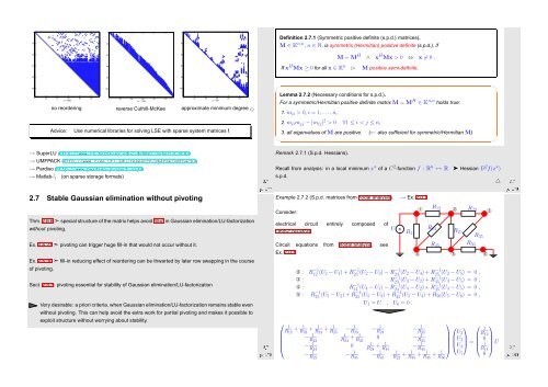
0 20 40 60 80 100
0
20
0
20
0
20
Definition 2.7.1 (Symmetric positive definite (s.p.d.) matrices).
M ∈ K n,n , n ∈ N, is symmetric (Hermitian) positive definite (s.p.d.), if
40
40
40
M = M H ∧ x H Mx > 0 ⇔ x ≠ 0 .
60
60
60
If x H Mx ≥ 0 for all x ∈ K n ✄ M positive semi-definite.
80
80
80
100
100
100
nz = 2580
0 20 40 60 80 100
0 20 40 60 80 100
nz = 891
nz = 1299
no reordering
reverse Cuthill-McKee approximate minimum degree ✸
Advice: Use numerical libraries for solving LSE with sparse system matrices !
✬
Lemma 2.7.2 (Necessary conditions for s.p.d.).
For a symmetric/Hermitian positive definite matrix M = M H ∈ K n,n holds true:
1. m ii > 0, i = 1, ...,n,
2. m ii m jj − |m ij | 2 > 0 ∀1 ≤ i < j ≤ n,
3. all eigenvalues of M are positive. (← also sufficient for symmetric/Hermitian M)
✫
✩
✪
→ SuperLU (http://www.cs.berkeley.edu/~demmel/SuperLU.html)
→ UMFPACK (http://www.cise.ufl.edu/research/sparse/umfpack/)
→ Pardiso
Ôº½ ¾º
(http://www.pardiso-project.org/)
→ Matlab-\ (on sparse storage formats)
2.7 Stable Gaussian elimination without pivoting
Remark 2.7.1 (S.p.d. Hessians).
Recall from analysis: in a local minimum x ∗ of a C 2 -function f : R n ↦→ R ➤ Hessian D 2 f(x ∗ )
s.p.d.
Example 2.7.2 (S.p.d. matrices from nodal analysis). → Ex. 2.0.1
△
Ôº½ ¾º
Thm. 2.6.6 ➣ special structure of the matrix helps avoid fill-in in Gaussian elimination/LU-factorization
without pivoting.
Consider:
electrical circuit entirely composed of
Ohmic resistors.
U
➀
R 12 ➁ R 23 ➂
~ R 24
R 14
R 25
R 35
Ex. 2.6.21 ➣ pivoting can trigger huge fill-in that would not occur without it.
Ex. 2.6.30 ➣ fill-in reducing effect of reordering can be thwarted by later row swapping in the course
of pivoting.
Sect. 2.5.3: pivoting essential for stability of Gaussian elimination/LU-factorization
Very desirable: a priori criteria, when Gaussian elimination/LU-factorization remains stable even
without pivoting. This can help avoid the extra work for partial pivoting and makes it possible to
exploit structure without worrying about stability.
Ôº½ ¾º
Circuit equations from nodal analysis, see
Ex. 2.0.1:
R45
R 56
➃ ➄ ➅
➁ : R12 −1 (U 2 − U 1 ) + R23 −1 (U 2 − U 3 ) − R24 −1 (U 2 − U 4 ) + R25 −1 (U 2 − U 5 ) = 0 ,
➂ :
R23 −1 (U 3 − U 2 ) + R35 −1 (U 3 − U 5 ) = 0 ,
➃ :
R14 −1 (U 4 − U 1 ) − R24 −1 (U 4 − U 2 ) + R45 −1 (U 4 − U 5 ) = 0 ,
➄ : R25 −1 (U 5 − U 2 ) + R35 −1 (U 5 − U 3 ) + R45 −1 (U 5 − U 4 ) + R 56 (U 5 − U 6 ) = 0 ,
U 1 = U , U 6 = 0 .
⎛
1
R + 12 R 1 + 23 R 1 + 24 R 1 − 25 R 1 − 23 R 1
− 1 ⎞
⎛ ⎞ ⎛ ⎞
1
24 R 25
− R 1
1
23 R + 1
23 R 0 − 1
U 2 R 35 R 35
⎜
⎝ −R 1
0 1
24 R + 1
24 R − 1
⎜U 3
12
⎟
⎟ ⎝
45 R 45 ⎠
U 4 ⎠ = 0
⎜
⎝
1 ⎟
−R 1
− 1
25 R − 1 1
35 R 45 R + 1
22 R + 1
35 R + 1
R ⎠ U
14
U 5 0
45 R 56
Ôº½¼ ¾º