Numerical Methods Contents - SAM

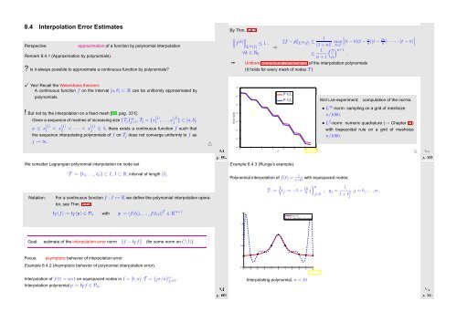
8.4 Interpolation Error Estimates
Perspective
approximation of a function by polynomial interpolation
Remark 8.4.1 (Approximation by polynomials).
? Is it always possible to approximate a continuous function by polynomials?
By Thm. 8.4.2:
∥
∥f (k)∥ ∥ ∥L ≤ 1 , ‖f − p‖ L ∞ (I) ≤ 1
∣ ∞ (I)
(1 + n)! max ∣
∣(t − 0)(t −
t∈I
n π)(t − 2π ∣∣
n ) · · · · · (t − π)
⇒
∀k ∈ N 0
≤ 1 ( π
) n+1
.
n + 1 n
➙ Uniform exponential convergence of the interpolation polynomials
(It holds for every mesh of nodes T )
̌ Yes! Recall the Weierstrass theorem:
A continuous function f on the interval [a,b] ⊂ R can be uniformly approximated by
polynomials.
10 −2
||f−p n
|| ∞
MATLAB-experiment:
computation of the norms.
10 0 n
! But not by the interpolation on a fixed mesh [32, pag. 331]:
Given a sequence of meshes of increasing size {T j } ∞ j=1 , T j = {x (j)
1 ,...,x(j) j } ⊂ [a,b],
a ≤ x (j)
1 < x (j)
2 < · · · < x (j)
j ≤ b, there exists a continuous function f such that
the sequence interpolating polynomials of f on T j does not converge uniformly to f as
j → ∞.
△
Ôº½ º
Error norm
10 −4
10 −6
10 −8
10 −10
10 −12
10 −14
||f−p n
|| 2
Fig. 100
2 4 6 8 10 12 14 16
• L ∞ -norm: sampling on a grid of meshsize
π/1000.
• L 2 -norm: numeric quadrature (→ Chapter 10)
with trapezoidal rule on a grid of meshsize
π/1000.
Ôº¿ º ✸
We consider Lagrangian polynomial interpolation on node set
Example 8.4.3 (Runge’s example).
Notation:
T := {t 0 ,...,t n } ⊂ I, I ⊂ R, interval of length |I|.
For a continuous function f : I ↦→ K we define the polynomial interpolation operator,
see Thm. 8.2.2
Polynomial interpolation of f(t) = 1
1+t2 with equispaced nodes:
{ } n
T := t j := −5 + 10
n j , y j = 1
j=0 1 + t 2 .j = 0, ...,n .
j
I T (f) := I T (y) ∈ P n with y := (f(t 0 ), ...,f(t n )) T ∈ K n+1 .
2
1/(1+x 2 )
Interpolating polynomial
1.5
✗
✖
Goal: estimate of the interpolation error norm ‖f − I T f‖ (for some norm on C(I)).
✔
✕
1
0.5
Focus:
asymptotic behavior of interpolation error
0
Example 8.4.2 (Asymptotic behavior of polynomial interpolation error).
Interpolation of f(t) = sint on equispaced nodes in I = [0, π]: T = {jπ/n} n j=0 .
Interpolation polynomial p := I T f ∈ P n .
Ôº¾ º
−0.5
−5 −4 −3 −2 −1 0 1 2 3 4 5
Fig. 101
Interpolating polynomial, n = 10
Ôº º