Numerical Methods Contents - SAM

f
f
• line 9: estimate for global error by summing up moduli of local error contributions,
• line 10: terminate, once the estimated total error is below the relative or absolute error threshold,
• line 13 otherwise, add midpoints of mesh intervals with large error contributions according to
(10.6.3) to the mesh and continue.
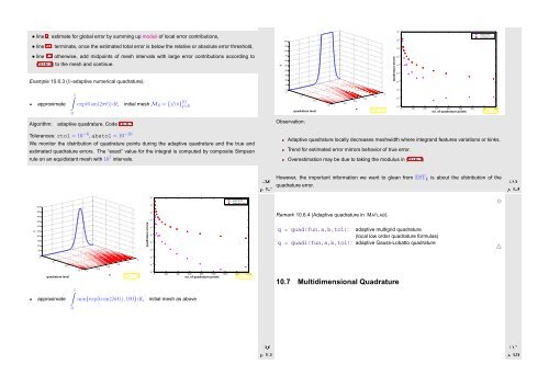
Example 10.6.3 (h-adaptive numerical quadrature).
100
90
80
70
60
50
40
30
20
10
quadrature errors
10 0
10 −1
10 −2
10 −3
10 −4
10 −5
exact error
estimated error
approximate
∫1
0
exp(6 sin(2πt)) dt, initial mesh M 0 = {j/10} 10
j=0
0
0
5
10
quadrature level
15
1
0.8
0.6
x
0.4
0
0.2
Fig. 120
10 1 no. of quadrature points
10 −6
10 −7
10 −8
0 100 200 300 400 500 600 700 800
Fig. 121
Algorithm: adaptive quadrature, Code 10.6.1
Observation:
Tolerances: rtol = 10 −6 , abstol = 10 −10
We monitor the distribution of quadrature points during the adaptive quadrature and the true and
estimated quadrature errors. The “exact” value for the integral is computed by composite Simpson
rule on an equidistant mesh with 10 7 intervals.
Ôº½ ½¼º
Adaptive quadrature locally decreases meshwidth where integrand features variations or kinks.
Trend for estimated error mirrors behavior of true error.
Overestimation may be due to taking the modulus in (10.6.1)
However, the important information we want to glean from EST k is about the distribution of the
quadrature error.
Ôº½ ½¼º
500
10 0
exact error
estimated error
✸
450
400
350
10 −1
10 −2
Remark 10.6.4 (Adaptive quadrature in MATLAB).
300
250
200
150
100
50
quadrature errors
10 −3
10 −4
10 −5
10 −6
q = quad(fun,a,b,tol): adaptive multigrid quadrature
(local low order quadrature formulas)
q = quadl(fun,a,b,tol): adaptive Gauss-Lobatto quadrature
△
0
0
0
5
0.2
0.4
10
0.6
0.8
15
1
x
quadrature level
Fig. 118
∫1
approximate min{exp(6 sin(2πt)), 100} dt,
10 1 no. of quadrature points
10 −7
10 −8
10 −9
0 200 400 600 800 1000 1200 1400 1600
initial mesh as above
Fig. 119
10.7 Multidimensional Quadrature
0
Ôº½ ½¼º
Ôº¾¼ ½¼º