Numerical Methods Contents - SAM

Two-dimensional trigonometric basis of C m,n :
}
tensor product matrices
{(F m ) :,j (F n ) T :,l , 1 ≤ j ≤ m, 1 ≤ l ≤ n . (7.2.13)
10
Original
10
Blurred image
Basis transform: for y j1 ,j 2
∈ C, 0 ≤ j 1 < m, 0 ≤ j 2 < n compute (nested DFTs !)
20
20
c k1 ,k 2
=
m−1 ∑
n−1 ∑
j 1 =0 j 2 =0
y j1 ,j 2
ω j 1k 1
m ω j 2k 2
n , 0 ≤ k 1 < m, 0 ≤ k 2 < n .
30
40
50
30
40
50
MATLAB function: fft2(Y) .
60
60
70
70
80
80
Two-dimensional DFT by nested one-dimensional DFTs (7.2.8):
90 Fig. 96
120
20 40 60 80 100
90 Fig. 97
120
20 40 60 80 100
Here:
fft2(Y) = fft(fft(Y).’).’
.’ simply transposes the matrix (no complex conjugation)
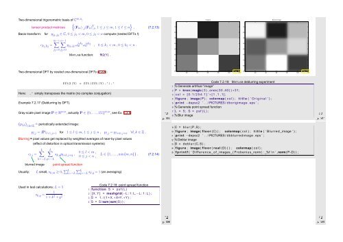
Example 7.2.17 (Deblurring by DFT).
Gray-scale pixel image P ∈ R m,n , actually P ∈ {0, ...,255} m,n , see Ex. 5.3.9.
( )
pl,k ˆ= periodically extended image:
l,k∈Z
p l,j = (P) l+1,j+1 for 1 ≤ l ≤ m, 1 ≤ j ≤ n , p l,j = p l+m,j+n ∀l,k ∈ Z .
Blurring = pixel values get replaced by weighted averages of near-by pixel values
c l,j =
(effect of distortion in optical transmission systems)
L∑
blurred image
L∑
k=−L q=−L
s k,q p l+k,j+q ,
point spread function
0 ≤ l < m ,
0 ≤ j < n ,
L ∈ {1, . ..,min{m, n}} . (7.2.14)
Ôº º¾
Code 7.2.19: MATLAB deblurring experiment
1 % Generate artifical “image”
2 P = kron ( magic ( 3 ) , ones (30 ,40) ) ∗31;
3 c o l = [ 0 : 1 / 2 5 4 : 1 ] ’ ∗ [ 1 , 1 , 1 ] ;
4 figure ; image (P) ; colormap ( c o l ) ; t i t l e ( ’ O r i g i n a l ’ ) ;
5 p r i n t −depsc2 ’ . . / PICTURES/ dborigimage . eps ’ ;
Ôº º¾
6 % Generate point spread function
7 L = 5 ; S = psf ( L ) ;
8 % Blur image
9 C = b l u r (P, S) ;
10 figure ; image ( f l o o r (C) ) ; colormap ( c o l ) ; t i t l e ( ’ Blurred image ’ ) ;
11 p r i n t −depsc2 ’ . . / PICTURES/ dbblurredimage . eps ’ ;
12 % Deblur image
13 D = deblur (C,S) ;
14 figure ; image ( f l o o r ( real (D) ) ) ; colormap ( c o l ) ;
15 f p r i n t f ( ’ D i f f e r e n c e o f images ( Frobenius norm ) : %f \ n ’ ,norm(P−D) ) ;
Usually:
L small, s k,m ≥ 0, ∑ L
k=−L
∑ Lq=−L
s k,q = 1 (an averaging)
Code 7.2.18: point spread function
Used in test calculations: L = 5
1 function S = psf ( L )
1
s k,q =
1 + k 2 + q 2 . 2 [ X,Y] = meshgrid(−L : 1 : L,−L : 1 : L ) ;
3 S = 1 . / ( 1 +X.∗X+Y.∗Y) ;
4 S = S /sum(sum(S) ) ;
Ôº º¾
Ôº º¾