Numerical Methods Contents - SAM

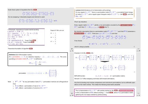
Scale linear system of equations from Ex. 2.3.1:
( )( )( )
2 /ǫ 0 ǫ 1 x1
=
0 1 1 1 x 2
( )( )
2 2/ǫ x1
=
1 1 x 2
( ) 2 /ǫ
1
No row swapping, if absolutely largest pivot element is used:
( ) ( ) ( ) ( )( )
2 2/ǫ 1 0 2 2/ǫ · 1 0 2 2/ǫ
=
=
1 1 1 1 0 1 − 2/ǫ 1 1 0 −2/ǫ
in M .
✬
Lemma 2.3.2 (Existence of LU-factorization with pivoting).
For any regular A ∈ K n,n there is a permutation matrix P ∈ K n,n , a normalized lower triangular
matrix L ∈ K n,n , and a regular upper triangular matrix U ∈ K n,n (→ Def. 2.2.1), such that
PA = LU .
✫
Proof. (by induction)
✩
✪
Every regular matrix A ∈ K n,n admits a row permutation encoded by the permutation matrix P ∈
K n,n , such that A ′ := (A) 1:n−1,1:n−1 is regular (why ?).
1 % Example: importance of scale-invariant pivoting
2 e p s i l o n = 5.0E−17;
3 A = [ e p s i l o n , 1 ; 1 , 1 ] ; b = [ 1 ; 2 ] ;
4 D = [ 1 / epsilon , 0 ; 0 , 1 ] ;
5 A = D∗A ; b = D∗b ;
6 x1 = A \ b ,
7 x2 =gausselim (A, b ) , % see Code 2.1.5
8 [ L ,U] = l u f a k (A) ; % see Code 2.2.1
9 z = L \ b ; x3 = U\ z ,
Theoretical foundation of algorithm 2.3.5:
Ouput of MATLAB run:
x1 = 1
1
x2 = 0
1
x3 = 0
1
Ôº½¼½ ¾º¿
By induction assumption there is a permutation matrix P ′ ∈ K n−1,n−1 such that P ′ A ′ possesses a
LU-factorization A ′ = L ′ U ′ . There are x,y ∈ K n−1 , γ ∈ K such that
( ) ( ) (
P ′ 0 P ′ 0 A ′
) (
x L ′ U ′ ) (
x L ′
)( )
0 U d
PA =
0 1 0 1 y T =
γ y T =
γ c T ,
1 0 α
if we choose
which is always possible.
d = (L ′ ) −1 x , c = (u ′ ) −T y , α = γ − c T d ,
✷
Ôº½¼¿ ¾º¿
Definition 2.3.1 (Permutation matrix).
An n-permutation, n ∈ N, is a bijective mapping π : {1, ...,n} ↦→ {1, ...,n}. The corresponding
permutation matrix P π ∈ K n,n is defined by
{
1 , if j = π(i) ,
(P π ) ij =
0 else.
⎛ ⎞
1 0 0 0
permutation (1, 2, 3, 4) ↦→ (1, 3, 2, 4) ˆ= P = ⎜0 0 1 0
⎟
⎝0 1 0 0⎠ .
0 0 0 1
Example 2.3.6 (Ex. 2.3.2 cnt’d).
⎛
A = ⎝ 1 2 2
⎞ ⎛
2 −7 2 ⎠ →
➊ ⎝ 2 −7 2
⎞ ⎛
1 2 2 ⎠ →
➋ ⎝ 2 −7 2
⎞ ⎛
0 5.5 1 ⎠ →
➌ ⎝ 2 −7 2
⎞ ⎛
0 27.5 −1 ⎠ →
➍ ⎝ 2 −7 2
⎞
0 27.5 −1 ⎠
1 24 0 1 24 0 0 27.5 −1 0 5.5 1 0 0 1.2
⎛
U = ⎝ 2 −7 2
⎞ ⎛
0 27.5 −1 ⎠, L = ⎝ 1 0 0
⎞ ⎛
0.5 1 0 ⎠ , P = ⎝ 0 1 0
⎞
0 0 1 ⎠ .
0 0 1.2
0.5 0.2 1 1 0 0
MATLAB function: [L,U,P] = lu(A) (P = permutation matrix)
✸
Remark 2.3.7 (Row swapping commutes with forward elimination).
Note:
P H = P −1 for any permutation matrix P (→ permutation matrices are orthogonal/unitary)
P π A effects π-permutation of rows of A ∈ K n,m
AP π effects π-permutation of columns of A ∈ K m,n
Ôº½¼¾ ¾º¿
Any kind of pivoting only involves comparisons and row/column permutations, but no arithmetic operations
on the matrix entries. This makes the following observation plausible:
The LU-factorization of A ∈ K n,n with partial pivoting by Alg. 2.3.5 is numerically equivalent
to the LU-factorization of PA without pivoting (→ Code 2.2.1), when P is a permutation matrix
gathering the row swaps entailed by partial pivoting.
Ôº½¼ ¾º¿