

Numerical Methods Contents - SAM
Numerical Methods Contents - SAM
Numerical Methods Contents - SAM

You also want an ePaper? Increase the reach of your titles
YUMPU automatically turns print PDFs into web optimized ePapers that Google loves.
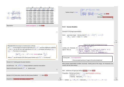
1 2 3<br />
k ρ (k)<br />
EV ρ (k)<br />
EW ρ (k)<br />
EV ρ (k)<br />
EW ρ (k)<br />
EV ρ (k)<br />
EW<br />
∥ ∥ ∥∥z (k) ∥∥<br />
22 0.9102 0.9007 0.5000 0.5000 0.9900 0.9781<br />
ρ (k) − s·,n<br />
EV := 23 0.9092 0.9004 0.5000 0.5000 0.9900 0.9791<br />
∥<br />
∥<br />
∥z (k−1) ∥∥<br />
,<br />
24 0.9083 0.9001 0.5000 0.5000 0.9901 0.9800<br />
− s·,n<br />
25 0.9075 0.9000 0.5000 0.5000 0.9901 0.9809<br />
ρ (k)<br />
EW := |ρ A(z (k) ) − λ n |<br />
|ρ A (z (k−1) ) − λ n | . 26 0.9068 0.8998 0.5000 0.5000 0.9901 0.9817<br />
27 0.9061 0.8997 0.5000 0.5000 0.9901 0.9825<br />
28 0.9055 0.8997 0.5000 0.5000 0.9901 0.9832<br />
29 0.9049 0.8996 0.5000 0.5000 0.9901 0.9839<br />
30 0.9045 0.8996 0.5000 0.5000 0.9901 0.9844<br />
Observation: linear convergence (→ Def. 3.1.4)<br />
“relative change” ≤ tol:<br />
5.3.2 Inverse Iteration<br />
⎧<br />
∥<br />
∥z<br />
⎪⎨<br />
(k) − z (k−1)∥ ∥ ≤ (1/L − 1)tol ,<br />
∥<br />
∥Az (k)∥ ∥ ∥<br />
∥Az (k−1)∥ ∣<br />
∥ ∣∣∣∣<br />
⎪⎩<br />
∥<br />
∣ ∥<br />
∥z (k) ∥∥ −<br />
∥<br />
∥<br />
∥z (k−1) ∥∥ ≤ (1/L − 1)tol see (3.1.7) .<br />
Estimated rate of convergence<br />
△<br />
✸<br />
Example 5.3.9 (Image segmentation).<br />
Ôº¾ º¿<br />
Given: grey-scale image: intensity matrix P ∈ {0,...,255} m,n , m, n ∈ N<br />
((P) ij ↔ pixel, 0 ˆ= black, 255 ˆ= white)<br />
Ôº¾ º¿<br />
✬<br />
Theorem 5.3.2 (Convergence of direct power method).<br />
Let λ n > 0 be the largest (in modulus) eigenvalue of A ∈ K n,n and have (algebraic) multiplicity<br />
1. Let v,y be the left and right eigenvectors of A for λ n normalized according to ‖y‖ 2 =<br />
‖v‖ 2 = 1. Then there is convergence<br />
∥<br />
∥Az (k)∥ ∥ ∥2 → λ n , z (k) → ±v linearly with rate |λ n−1|<br />
,<br />
|λ n |<br />
✫<br />
where z (k) are the iterates of the direct power iteration and y H z (0) ≠ 0 is assumed.<br />
Remark 5.3.7 (Initial guess for power iteration).<br />
roundoff errors ➤ y H z (0) ≠ 0 always satisfied in practical computations<br />
Usual (not the best!) choice for x (0) = random vector<br />
Remark 5.3.8 (Termination criterion for direct power iteration). (→ Sect. 3.1.2)<br />
Adaptation of a posteriori termination criterion (3.2.7)<br />
✩<br />
✪<br />
△<br />
Ôº¾ º¿<br />
Code 5.3.10: loading and displaying an image<br />
1 M = imread ( ’ eth .pbm ’ ) ;<br />
Loading and displaying images<br />
in MATLAB ✄ 3 f p r i n t f ( ’%dx%d grey scale p i x e l image \ n ’ ,m, n ) ;<br />
2 [m, n ] = size (M) ;<br />
4 figure ; image (M) ; t i t l e ( ’ETH view ’ ) ;<br />
5 c o l = [ 0 : 1 / 2 1 5 : 1 ] ’ ∗ [ 1 , 1 , 1 ] ; colormap ( c o l ) ;<br />
(Fuzzy) task:<br />
Local segmentation<br />
Find connected patches of image of the same shade/color<br />
More general segmentation problem (non-local): identify parts of the image, not necessarily connected,<br />
with the same texture.<br />
Next: Statement of (rigorously defined) problem, cf. Sect. 2.5.2:<br />
Ôº¾ º¿<br />
✎ notation: p k := (P) ij , if k = index(pixel i,j ) = (i − 1)n + j, k = 1,...,N := mn<br />
Preparation: Numbering of pixels 1 . ..,mn, e.g, lexicographic numbering:<br />
pixel set V := {1....,nm}<br />
indexing: index(pixel i,j ) = (i − 1)n + j


