Numerical Methods Contents - SAM

Then store G ij (a,b) as triple (i,j, ρ)
The rationale for this convention is to curb the impact of roundoff errors.
Fill-in for QR-decomposition ?
bandwidth
✗
✖
A ∈ C n,n with QR-decomposition A = QR ⇒ m(R) ≤ m(A) (→ Def. 2.6.4)
Example 2.8.14 (QR-based solution of tridiagonal LSE).
✔
✕
Storing orthogonal transformation matrices is usually inefficient !
Algorithm 2.8.11 (Solving linear system of equations by means of QR-decomposition).
Ax = b :
1 QR-decomposition A = QR, computational costs 2 3 n3 + O(n 2 ) (about twice
as expensive as LU-decomposition without pivoting)
2 orthogonal transformation z = Q H b, computational costs 4n 2 + O(n) (in the
case of compact storage of reflections/rotations)
3 Backward substitution, solve Rx = z, computational costs 1 2n(n + 1)
△
Ôº¾¼ ¾º
Elimination of Sub-diagonals by n − 1 successive Givens rotations:
⎛
⎞ ⎛
⎞
⎛
⎞
∗ ∗ 0 0 0 0 0 0 ∗ ∗ ∗ 0 0 0 0 0
∗ ∗ ∗ 0 0 0 0 0
∗ ∗ ∗ 0 0 0 0 0
0 ∗ ∗ 0 0 0 0 0
0 ∗ ∗ ∗ 0 0 0 0
0 ∗ ∗ ∗ 0 0 0 0
0 ∗ ∗ ∗ 0 0 0 0
0 0 ∗ ∗ ∗ 0 0 0
0 0 ∗ ∗ ∗ 0 0 0
G 12
0 0 0 ∗ ∗ ∗ 0 0
−−→
0 0 ∗ ∗ ∗ 0 0 0
G 23 G n−1,n
0 0 0 ∗ ∗ ∗ 0 0
−−→ · · · −−−−−→
0 0 0 ∗ ∗ ∗ 0 0
0 0 0 0 ∗ ∗ ∗ 0
⎜
0 0 0 0 ∗ ∗ ∗ 0
⎟ ⎜
0 0 0 0 ∗ ∗ ∗ 0
⎟
⎜
0 0 0 0 0 ∗ ∗ ∗
⎟
⎝0 0 0 0 0 ∗ ∗ ∗⎠
⎝0 0 0 0 0 ∗ ∗ ∗⎠
⎝0 0 0 0 0 0 ∗ ∗⎠
0 0 0 0 0 0 ∗ ∗ 0 0 0 0 0 0 ∗ ∗
0 0 0 0 0 0 0 ∗
MATLAB code (c,d,e,b = column vectors of length n, n ∈ N, e(n),c(n) not used):
⎛
⎞
d 1 c 1 0 ... 0
e 1 d 2 c 2 .
A =
⎜ 0 e 2 d 3 c 3
⎟ ↔ spdiags([e,d,c],[-1 0 1],n,n)
⎝ . . .. . .. . .. c n−1 ⎠
0 ... 0 e n−1 d n
Ôº¾½½ ¾º
✬
✌ Computing the generalized QR-decomposition A = QR by means of Householder reflections
or Givens rotations is (numerically stable) for any A ∈ C m,n .
✌ For any regular system matrix an LSE can be solved by means of
✫
in a stable manner.
QR-decomposition + orthogonal transformation + backward substitution
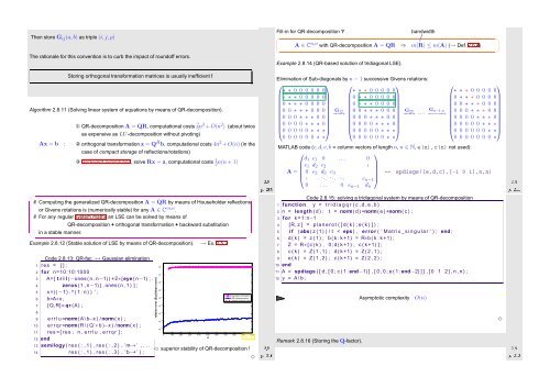
Example 2.8.12 (Stable solution of LSE by means of QR-decomposition). → Ex. 2.5.2
Code 2.8.13: QR-fac. ↔ Gaussian elimination
1 res = [ ] ;
2 for n=10:10:1000
3 A=[ t r i l (−ones ( n , n−1) ) +2∗[eye ( n−1) ; . . .
4 zeros ( 1 , n−1) ] , ones ( n , 1 ) ] ;
5 x=(( −1) . ^ ( 1 : n ) ) ’ ;
6 b=A∗x ;
7 [Q,R]= qr (A) ;
8
9 e r r l u =norm(A \ b−x ) / norm( x ) ;
10 e r r q r =norm(R \ ( Q’∗ b )−x ) / norm( x ) ;
11 res =[ res ; n , e r r l u , e r r q r ] ;
12 end
13 semilogy ( res ( : , 1 ) , res ( : , 2 ) , ’m−∗ ’ , . . .
14 res ( : , 1 ) , res ( : , 3 ) , ’ b−+ ’ ) ;
relative error (Euclidean norm)
10 0
10 −2
10 −4
10 −6
Gaussian elimination
10 −8
QR−decomposition
relative residual norm
10 −10
10 −12
10 −14
10 −16
0 100 200 300 400 500 600 700 800 900 1000
n
Fig. 25
✩
✪
Ôº¾½¼ ¾º
Remark 2.8.16 (Storing the Q-factor).
✁ superior stability of QR-decomposition !
✸
Code 2.8.15: solving a tridiagonal system by means of QR-decomposition
1 function y = t r i d i a g q r ( c , d , e , b )
2 n = length ( d ) ; t = norm( d ) +norm( e ) +norm( c ) ;
3 for k =1:n−1
4 [R, z ] = p l a n e r o t ( [ d ( k ) ; e ( k ) ] ) ;
5 i f ( abs ( z ( 1 ) ) / t < eps ) , error ( ’ M a trix s i n g u l a r ’ ) ; end ;
6 d ( k ) = z ( 1 ) ; b ( k : k +1) = R∗b ( k : k +1) ;
7 Z = R∗[ c ( k ) , 0 ; d ( k +1) , c ( k +1) ] ;
8 c ( k ) = Z ( 1 , 1 ) ; d ( k +1) = Z ( 2 , 1 ) ;
9 e ( k ) = Z ( 1 , 2 ) ; c ( k +1) = Z ( 2 , 2 ) ;
10 end
11 A = spdiags ( [ d , [ 0 ; c ( 1 : end−1) ] , [ 0 ; 0 ; e ( 1 : end−2) ] ] , [ 0 1 2 ] , n , n ) ;
12 y = A \ b ;
Asymptotic complexity
O(n)
✸
Ôº¾½¾ ¾º