

Numerical Methods Contents - SAM
Numerical Methods Contents - SAM
Numerical Methods Contents - SAM

You also want an ePaper? Increase the reach of your titles
YUMPU automatically turns print PDFs into web optimized ePapers that Google loves.
f<br />
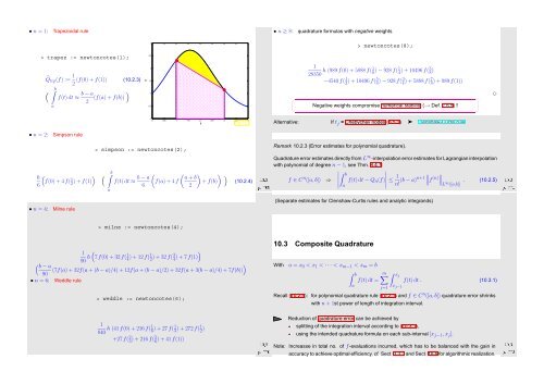
• n = 1:<br />
Trapezoidal rule<br />
• n ≥ 8:<br />
quadrature formulas with negative weights<br />
3<br />
> newtoncotes(8);<br />
> trapez := newtoncotes(1);<br />
̂Q trp (f) := 1 (f(0) + f(1)) (10.2.3)<br />
2<br />
( ∫ b<br />
a<br />
f(t) dt ≈ b − a<br />
2 (f(a) + f(b)) )<br />
2.5<br />
000000000000000<br />
111111111111111<br />
000000000000000<br />
111111111111111<br />
2<br />
000000000000000<br />
111111111111111<br />
000000000000000<br />
111111111111111<br />
000000000000000<br />
111111111111111<br />
000000000000000<br />
111111111111111<br />
1.5<br />
000000000000000<br />
111111111111111<br />
000000000000000<br />
111111111111111<br />
1<br />
X<br />
000000000000000<br />
000000000000000<br />
000000000000000<br />
111111111111111<br />
111111111111111<br />
111111111111111<br />
000000000000000<br />
111111111111111<br />
000000000000000<br />
111111111111111<br />
000000000000000<br />
111111111111111<br />
0.5<br />
000000000000000<br />
111111111111111<br />
000000000000000<br />
111111111111111<br />
000000000000000<br />
111111111111111<br />
0<br />
000000000000000<br />
111111111111111<br />
0 0.5 1000000000000000<br />
111111111111111<br />
1.5 2 2.5 3 3.5 4<br />
t<br />
Fig. 111<br />
✗<br />
✖<br />
1<br />
28350 h (989f(0) + 5888 f(1 8 ) − 928 f(1 4 ) + 10496f(3 8 )<br />
−4540f( 2 1) + 10496f(5 8 ) − 928f(3 4 ) + 5888 f(7 8 ) + 989 f(1))<br />
✸<br />
Negative weights compromise numerical stability (→ Def. 2.5.5) !<br />
Alternative: If t j = Chebychev nodes (8.5.1) ➤ Clenshaw-Curtis rule<br />
✔<br />
✕<br />
• n = 2:<br />
Simpson rule<br />
h<br />
(<br />
)<br />
f(0) + 4f( 1 6<br />
2 ) + f(1)<br />
> simpson := newtoncotes(2);<br />
( ∫ b<br />
a<br />
f(t) dt ≈ b − a (<br />
f(a) + 4 f<br />
6<br />
( a + b<br />
2<br />
)<br />
+ f(b)<br />
) )<br />
Ôº ½¼º¾<br />
(10.2.4)<br />
Remark 10.2.3 (Error estimates for polynomial quadrature).<br />
Ôº½ ½¼º¾<br />
∣ ≤ 1 ∥ n! (b − a)n+1 ∥ ∥f<br />
(n) ∥L . ∞ ([a,b]) (10.2.5)<br />
Quadrature error estimates directly from L ∞ -interpolation error estimates for Lagrangian interpolation<br />
with polynomial of degree n − 1, see Thm. 8.4.1:<br />
∫ f ∈ C n b<br />
([a,b]) ⇒<br />
f(t) dt − Q<br />
∣<br />
n (f) ∣<br />
a<br />
• n = 4:<br />
Milne rule<br />
(Separate estimates for Clenshaw-Curtis rules and analytic integrands)<br />
△<br />
> milne := newtoncotes(4);<br />
1<br />
(<br />
)<br />
90 h 7f(0) + 32 f( 1 4 ) + 12f(1 2 ) + 32 f(3 4 ) + 7 f(1)<br />
( b − a<br />
)<br />
90 (7f(a) + 32f(a + (b − a)/4) + 12f(a + (b − a)/2) + 32f(a + 3(b − a)/4) + 7f(b))<br />
• n = 6: Weddle rule<br />
> weddle := newtoncotes(6);<br />
10.3 Composite Quadrature<br />
With a = x 0 < x 1 < · · · < x m−1 < x m = b<br />
∫ b m∑<br />
∫ xj<br />
f(t) dt = f(t) dt . (10.3.1)<br />
a<br />
j=1<br />
x j−1<br />
Recall (10.2.5): for polynomial quadrature rule (10.2.1) and f ∈ C n ([a,b]) quadrature error shrinks<br />
with n + 1st power of length of integration interval.<br />
1<br />
840 h (41 f(0) + 216 f(1 6 ) + 27f(1 3 ) + 272 f(1 2 )<br />
Ôº¼<br />
+27f( 2 3 ) + 216 f(5 6 ) + 41 f(1))<br />
½¼º¾<br />
Reduction of quadrature error can be achieved by<br />
splitting of the integration interval according to (10.3.1),<br />
using the intended quadrature formula on each sub-interval [x j−1 , x j ].<br />
Note: Increasse in total no. of f-evaluations incurred, which has to be balanced with the gain in<br />
accuracy to achieve optimal efficiency, cf. Sect. 3.3.3 and Sect. 10.6 for algorithmic realization.<br />
Ôº¾ ½¼º¿


