Numerical Methods Contents - SAM

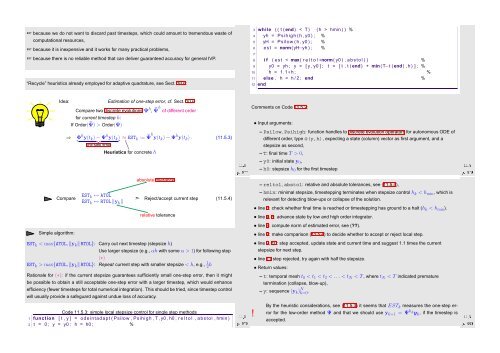
☞ because we do not want to discard past timesteps, which could amount to tremendous waste of
computational resources,
☞ because it is inexpensive and it works for many practical problems,
☞ because there is no reliable method that can deliver guaranteed accuracy for general IVP.
“Recycle” heuristics already employed for adaptive quadrature, see Sect. 10.6:
3 while ( ( t ( end ) < T ) ( h > hmin ) ) %
4 yh = Psihigh ( h , y0 ) ; %
5 yH = Psilow ( h , y0 ) ; %
6 est = norm( yH−yh ) ; %
7
8 i f ( est < max( r e l t o l ∗norm( y0 ) , a b s t o l ) ) %
9 y0 = yh ; y = [ y , y0 ] ; t = [ t , t ( end ) + min ( T−t ( end ) , h ) ] ; %
10 h = 1.1∗h ; %
11 else , h = h / 2 ; end %
12 end
Idea: Estimation of one-step error, cf. Sect. 10.6
Compare two discrete evolutions Ψ h , ˜Ψ h of different order
for current timestep h:
If Order(˜Ψ) > Order(Ψ)
⇒ Φ h y(t k ) − Ψ h y(t k ) ≈ EST
} {{ } k := ˜Ψ h y(t k ) − Ψ h y(t k ) . (11.5.3)
one-step error
Heuristics for concrete h
Ôº ½½º
Comments on Code 11.5.2:
• Input arguments:
– Psilow, Psihigh: function handles to discrete evolution operators for autonomous ODE of
different order, type @(y,h), expecting a state (column) vector as first argument, and a
Ôº ½½º
– h0: stepsize h 0 for the first timestep
stepsize as second,
– T: final time T > 0,
– y0: initial state y 0 ,
Compare
Simple algorithm:
EST k ↔ ATOL
EST k ↔ RTOL ‖y k ‖
absolute tolerance
➣ Reject/accept current step (11.5.4)
relative tolerance
EST k < max{ATOL, ‖y k ‖RTOL}: Carry out next timestep (stepsize h)
Use larger stepsize (e.g., αh with some α > 1) for following step
(∗)
EST k > max{ATOL, ‖y k ‖RTOL}: Repeat current step with smaller stepsize < h, e.g., 1 2 h
Rationale for (∗): if the current stepsize guarantees sufficiently small one-step error, then it might
be possible to obtain a still acceptable one-step error with a larger timestep, which would enhance
efficiency (fewer timesteps for total numerical integration). This should be tried, since timestep control
Ôº ½½º
Code 11.5.3: simple local stepsize control for single step methods
1 function [ t , y ] = odeintadapt ( Psilow , Psihigh , T , y0 , h0 , r e l t o l , abstol , hmin )
2 t = 0 ; y = y0 ; h = h0 ; %
will usually provide a safeguard against undue loss of accuracy.
!
– reltol, abstol: relative and absolute tolerances, see (11.5.4),
– hmin: minimal stepsize, timestepping terminates when stepsize control h k < h min , which is
relevant for detecting blow-ups or collapse of the solution.
• line 3: check whether final time is reached or timestepping has ground to a halt (h k < h min ).
• line 4, 5: advance state by low and high order integrator.
• line 6: compute norm of estimated error, see (??).
• line 8: make comparison (11.5.4) to decide whether to accept or reject local step.
• line 9, 10: step accepted, update state and current time and suggest 1.1 times the current
stepsize for next step.
• line 11 step rejected, try again with half the stepsize.
• Return values:
– t: temporal mesh t 0 < t 1 < t 2 < . .. < t N < T , where t N < T indicated premature
termination (collapse, blow-up),
– y: sequence (y k ) N k=0 .
By the heuristic considerations, see (11.5.3) it seems that EST k measures the one-step error
for the low-order method Ψ and that we should use y k+1 = Ψ h ky k , if the timestep is
accepted.
Ôº¼ ½½º