Numerical Methods Contents - SAM

1.3 Complexity/computational effort
complexity/computational effort of an algorithm :⇔ number of elementary operators
additions/multiplications
Crucial: dependence of (worst case) complexity of an algorithm on (integer) problem size parameters
(worst case ↔ maximum for all possible data)
Usually studied: asymptotic complexity ˆ= “leading order term” of complexity w.r.t large problem
size parameters
The usual choice of problem size parameters in numerical linear algebra is the number of independent
real variables needed to describe the input data (vector length, matrix sizes).
Q 2 = A 11 ∗ (B 12 − B 22 ) ,
Q 3 = A 22 ∗ (−B 11 + B 21 ) ,
Q 4 = (A 11 + A 12 ) ∗ B 22 ,
Q 5 = (−A 11 + A 21 ) ∗ (B 11 + B 12 ) ,
Q 6 = (A 12 − A 22 ) ∗ (B 21 + B 22 ) .
Beside a considerable number of matrix additions ( computational effort O(n 2 ) ) it takes only 7 multiplications
of matrices of size n/2 to compute C! Strassen’s algorithm boils down to the recursive
application of these formulas for n = 2 k , k ∈ N.
A refined algorithm of this type can achieve complexity O(n 2.36 ), see [7].
△
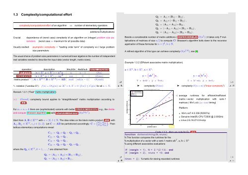
Example 1.3.2 (Efficient associative matrix multiplication).
operation description #mul/div #add/sub asymp. complexity
dot product (x ∈ R n ,y ∈ R n ) ↦→ x H y n n − 1 O(n)
tensor product (x ∈ R m ,y ∈ R n ) ↦→ xy H nm 0 O(mn)
Ôº½ ½º¿
matrix product (∗) (A ∈ R m,n ,B ∈ R n,k ) ↦→ AB mnk mk(n − 1) O(mnk)
✎ notation (“Landau-O”): f(n) = O(g(n)) ⇔ ∃C > 0, N > 0: |f(n)| ≤ Cg(n) for all n > N.
Remark 1.3.1 (“Fast” matrix multiplication).
(∗):
O(mnk) complexity bound applies to “straightforward” matrix multiplication according to
(1.2.1).
For m = n = k there are (sophisticated) variants with better asymptotic complexity, e.g., the divideand-conquer
Strassen algorithm [39] with asymptotic complexity O(n log 2 7 ):
Start from A,B ∈ K n,n with n = 2l, l ∈ N. The idea relies on the block matrix product ( (1.2.3) with
A ij ,B ij ∈ K l,l , i,j ∈ {1, 2}. Let C := AB be partiotioned accordingly: C = C11 C 22
C 21 C
). Then 22
tedious elementary computations reveal
a ∈ K m , b ∈ K n , x ∈ K n :
(
y = ab T) x .
average runtime (s)
T = a*b’; y = T*x;
➤
complexity O(mn)
tic−toc timing, mininum over 10 runs
slow evaluation
efficient evaluation
O(n)
10 0
O(n 2 )
10 −1
10 −2
10 −3
10 −4
10 −5
10 −6
10 0 10 1 10 2 10 3 10 4
problem size n
Fig. 1
10 1
Ôº¿ ½º¿
➤ complexity O(n + m) (“linear complexity”)
( )
y = a b T x .
t = b’*x; y = a*t;
✁ average runtimes for efficient/inefficient
matrix×vector multiplication with rank-1
matrices ( MATLABtic-toc timing)
Platform:
MATLAB7.4.0.336 (R2007a)
Genuine Intel(R) CPU T2500 @ 2.00GHz
Linux 2.6.16.27-0.9-smp
C 11 = Q 0 + Q 3 − Q 4 + Q 6 ,
C 21 = Q 1 + Q 3 ,
C 12 = Q 2 + Q 4 ,
C 22 = Q 0 + Q 2 − Q 1 + Q 5 ,
where the Q k ∈ K l,l , k = 1,...,7 are obtained from
Q 0 = (A 11 + A 22 ) ∗ (B 11 + B 22 ) ,
Q 1 = (A 21 + A 22 ) ∗ B 11 ,
Ôº¾ ½º¿
Code 1.3.3: MATLAB code for Ex. 1.3.2
1 function d o t t e n s t i m i n g (N, nruns )
2 % This function compares the runtimes for the
3 % multiplication of a vector with a rank-1 matrix ab T , a,b ∈ R n
4 % using different associative evaluations
5
6 i f ( nargin < 1) , N = 2 . ^ ( 2 : 1 3 ) ; end
Ôº ½º¿
7 i f ( nargin < 2) , nruns = 10; end
8
9 times = [ ] ; % matrix for storing recorded runtimes