Numerical Methods Contents - SAM

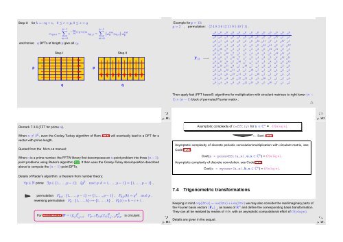
Step II: for k =: rq + s, 0 ≤ r < p, 0 ≤ s < q
∑p−1
c rq+s = e −2πi pq (rq+s)m p−1 ∑ (
z m,s = ω
ms )
n z m,s ω
mr
p
m=0
m=0
and hence q DFTs of length p give all c k .
p
Step I
q
p
Step II
q
Example for p = 13:
g = 2 , permutation: (2 4 8 3 6 12 11 9 5 10 7 1) .
F 13
−→
ω 0 ω 0 ω 0 ω 0 ω 0 ω 0 ω 0 ω 0 ω 0 ω 0 ω 0 ω 0 ω 0
ω 0 ω 2 ω 4 ω 8 ω 3 ω 6 ω 12 ω 11 ω 9 ω 5 ω 10 ω 7 ω 1
ω 0 ω 1 ω 2 ω 4 ω 8 ω 3 ω 6 ω 12 ω 11 ω 9 ω 5 ω 10 ω 7
ω 0 ω 7 ω 1 ω 2 ω 4 ω 8 ω 3 ω 6 ω 12 ω 11 ω 9 ω 5 ω 10
ω 0 ω 10 ω 7 ω 1 ω 2 ω 4 ω 8 ω 3 ω 6 ω 12 ω 11 ω 9 ω 5
ω 0 ω 5 ω 10 ω 7 ω 1 ω 2 ω 4 ω 8 ω 3 ω 6 ω 12 ω 11 ω 9
ω 0 ω 9 ω 5 ω 10 ω 7 ω 1 ω 2 ω 4 ω 8 ω 3 ω 6 ω 12 ω 11
ω 0 ω 11 ω 9 ω 5 ω 10 ω 7 ω 1 ω 2 ω 4 ω 8 ω 3 ω 6 ω 12
ω 0 ω 12 ω 11 ω 9 ω 5 ω 10 ω 7 ω 1 ω 2 ω 4 ω 8 ω 3 ω 6
ω 0 ω 6 ω 12 ω 11 ω 9 ω 5 ω 10 ω 7 ω 1 ω 2 ω 4 ω 8 ω 3
ω 0 ω 3 ω 6 ω 12 ω 11 ω 9 ω 5 ω 10 ω 7 ω 1 ω 2 ω 4 ω 8
ω 0 ω 8 ω 3 ω 6 ω 12 ω 11 ω 9 ω 5 ω 10 ω 7 ω 1 ω 2 ω 4
ω 0 ω 4 ω 8 ω 3 ω 6 ω 12 ω 11 ω 9 ω 5 ω 10 ω 7 ω 1 ω 2
△
Ôº¼½ º¿
Then apply fast (FFT based!) algorithms for multiplication with circulant matrices to right lower (n −
1) × (n − 1) block of permuted Fourier matrix .
△
Ôº¼¿ º¿
Remark 7.3.6 (FFT for prime n).
Asymptotic complexity of c=fft(y) for y ∈ C n =
O(n log n).
When n ≠ 2 L , even the Cooley-Tuckey algorithm of Rem. 7.3.5 will eventually lead to a DFT for a
vector with prime length.
Quoted from the MATLAB manual:
When n is a prime number, the FFTW library first decomposes an n-point problem into three (n − 1)-
point problems using Rader’s algorithm [33]. It then uses the Cooley-Tukey decomposition described
above to compute the (n − 1)-point DFTs.
← Sect. 7.2.1
Asymptotic complexity of discrete periodic convolution/multiplication with circulant matrix, see
Code 7.2.6:
Cost(z = pconvfft(u,x), u,x ∈ C n ) = O(n log n).
Asymptotic complexity of discrete convolution, see Code 7.2.8:
Cost(z = myconv(h,x), h,x ∈ C n ) = O(n log n).
Details of Rader’s algorithm: a theorem from number theory:
∀p ∈ N prime ∃g ∈ {1, ...,p − 1}: {g k mod p: k = 1, ...,p − 1} = {1,...,p − 1} ,
permutation P p,g : {1, . ..,p − 1} ↦→ {1, ...,p − 1} , P p,g (k) = g k mod p ,
reversing permutation P k : {1, ...,k} ↦→ {1, ...,k} , P k (i) = k − i + 1 .
For Fourier matrix F = (f ij ) p i,j=1 : P p−1P p,g (f ij
Ôº¼¾ º¿
) p i,j=2 PT p,g is circulant.
7.4 Trigonometric transformations
Keeping in mind exp(2πix) = cos(2πx)+i sin(2πx) we may also consider the real/imaginary parts of
the Fourier basis vectors (F n ) :,j as bases of R n and define the corresponding basis transformation.
They can all be realized by means of fft with an asymptotic computational effort of O(n log n).
Details are given in the sequel.
Ôº¼ º