Numerical Methods Contents - SAM

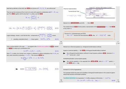
Note that by definition of the SVD, Def. 5.5.2, the columns of U 1 ,U 2 ,V 1 ,V 2 are orthonormal.
Then we use the invariance of the 2-norm of a vector with respect to multiplication with U = [U 1 ,u 2 ],
see Thm. 2.8.2, together with the fact that U is unitary, see Def. 2.8.1:
[ (U H) ]
[U 1 ,u 2 ] · 1
U H = I .
2
Practical implementation:
“numerical rank” test:
r = max{i: σ i /σ 1 > tol}
Code 6.2.1: Solving LSQ problem via SVD
1 function y = lsqsvd (A, b )
2 [U, S, V] = svd (A, 0 ) ;
3 sv = diag (S) ;
4 r = max( find ( sv / sv ( 1 ) > eps ) ) ;
5 y = V ( : , 1 : r ) ∗( diag ( 1 . / sv ( 1 : r ) ) ∗ . . .
6 (U( : , 1 : r ) ’∗b ) ) ;
Remark 6.2.2 (Pseudoinverse and SVD). → Rem. 6.0.4
( ) ( )
( ‖Ax − b‖ 2 =
∥ [U Σr 0 V H 1 U 2 ]
1
0 0 V2
H x − b
∥ =
Σr V1 H ∥
x
2
0
)
−
(
U H
1 b
U H 2 b )∥ ∥∥∥2
(6.2.2)
The solution formula (6.2.5) directly yields a representation of the pseudoinverse A + (→ Def. 6.0.2)
of any matrix A:
✬
✩
Logical strategy: choose x such that the first r components of
(
Σr V1 Hx
) ( )
U H
− 1 b
0 U H 2 b vanish:
Theorem 6.2.1 (Pseudoinverse and SVD).
If A ∈ K m,n has the SVD decomposition (6.2.1), then
A + = V 1 Σ −1 r U H 1
holds.
➣ (possibly underdetermined) r × n linear system Σ r V H 1 x = UH 1 b . (6.2.3)
Ôº½ º¾
✫
Ôº½ º¾
✪
△
To fix a unique solution in the case r < n we appeal to the minimal norm condition in (6.0.3): solution
x of (6.2.3) is unique up to contributions from
Ker(V H 1 ) = Im(V 1) ⊥ = Im(V 2 ) . (6.2.4)
Since V is unitary, the minimal norm solution is obtained by setting contributions from Im(V 2 ) to
zero, which amounts to choosing x ∈ Im(V 1 ). This converts (6.2.3) into
Remark 6.2.3 (Normal equations vs. orthogonal transformations method).
Superior numerical stability (→ Def. 2.5.5) of orthogonal transformations methods:
Use orthogonal transformations methods for least squares problems (6.0.3), whenever A ∈
R m,n dense and n small.
Σ r V
} 1 H {{ V } 1 z = U H 1 b ⇒
=I
z = Σ−1 r U H 1 b .
SVD/QR-factorization cannot exploit sparsity:
Use normal equations in the expanded form (6.1.3)/(6.1.4), when A ∈ R m,n sparse (→
Def. 2.6.1) and m, n big.
△
solution
∥ x = V 1 Σ −1 r U H ∥∥U
1 b , ‖r‖ 2 = H 2 b∥ . (6.2.5)
2
Example 6.2.4 (Fit of hyperplanes).
Ôº½ º¾
This example studies the power and versatility of orthogonal transformations in the context of (generalized)
least squares minimization problems.
Ôº¾¼ º¾
H = {x ∈ R d : c + n T x = 0} , ‖n‖ 2 = 1 . (6.2.6)
The Hesse normal form of a hyperplane H (= affine subspace of dimension d − 1) in R d is: