Numerical Methods Contents - SAM

Rewriting estimate of Thm. 2.5.9 with ∆b = 0,
ǫ r :=
‖x − ˜x‖
‖x‖
≤
cond(A)δ A
, δ
1 − cond(A)δ A := ‖∆A‖
A ‖A‖ . (2.5.8)
(2.5.8) ➣ If cond(A) ≫ 1, small perturbations in A can lead to large relative errors in the
solution of the LSE.
★
If cond(A) ≫ 1, a stable algorithm (→ Def. 2.5.5) can produce solutions
with large relative error !
✧
Example 2.5.8 (Conditioning and relative error).
→ Ex. 2.5.3 cnt’d
✥
✦
cond 2
(A)
140
120
100
80
60
40
20
0
0 50 100 150
n
200 250 300
Fig. 8
relative error (Euclidean norm)
10 0
10 −2
10 −4
10 −6
Gaussian elimination
10 −8
QR−decomposition
relative residual norm
10 −10
10 −12
10 −14
10 −16
0 100 200 300 400 500
n
600 700 800 900 1000
Fig. 9
Numerical experiment with nearly singular matrix
from Ex. 2.5.3
A = uv T + ǫI ,
cond(A)
10 20
10 19
10 18
10 17
10 16
u = 1 3 (1, 2, 3,...,10)T 10
,
−2
10 15
v = (−1, 1 2 , −1 3 , 1 4 , ..., 10 1 )T 10 −3
10 14
Ôº½¿¿ ¾º
10 13
10 −4
relative error
10 12
10 −14 10 −13 10 −12 10 −11 10 −10 10 −9 10 −8 10 −7 10 −6 10 −5
10−5
ε
Fig. 7 ✸
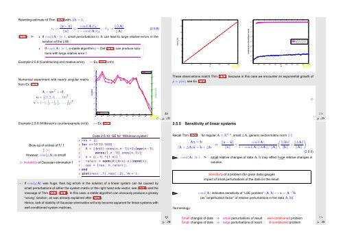
Example 2.5.9 (Wilkinson’s counterexample cnt’d). → Ex. 2.5.2
cond(A)
10 2
10 1
10 0
10 −1
relative error
These observations match Thm. 2.5.7, because in this case we encounter an exponential growth of
ρ = ρ(n), see Ex. 2.5.2.
2.5.5 Sensitivity of linear systems
✸
Ôº½¿ ¾º
Blow-up of entries of U !
↕ (∗)
However, cond 2 (A) is small!
✄ Instability of Gaussian elimination !
Code 2.5.10: GE for “Wilkinson system”
1 res = [ ] ;
2 for n=10:10:1000
3 A = [ t r i l (−ones ( n , n−1) ) +2∗[eye ( n−1) ;
4 zeros ( 1 , n−1) ] , ones ( n , 1 ) ] ;
5 x = (( −1) . ^ ( 1 : n ) ) ’ ;
6 r e l e r r = norm(A \ ( A∗x )−x ) / norm( x ) ;
7 res = [ res ; n , r e l e r r ] ;
8 end
9 plot ( res ( : , 1 ) , res ( : , 2 ) , ’m−∗ ’ ) ;
(∗) If cond 2 (A) was huge, then big errors in the solution of a linear system can be caused by
small perturbations of either the system matrix or the right hand side vector, see (2.5.6) and the
message of Thm. 2.5.9, (2.5.8). In this case, a stable algorithm can obviously produce a grossly
“wrong” solution, as was already explained after (2.5.8).
Hence, lack of stability of Gaussian elimination will only become apparent for linear systems with
well-conditioned system matrices.
Ôº½¿ ¾º
Recall Thm. 2.5.9:
Ax = b
(A + ∆A)˜x = b + ∆b
cond(A) ≫ 1 ➣
Terminology:
for regular A ∈ K n,n , small ∆A, generic vector/matrix norm ‖·‖
⇒
‖x − ˜x‖
‖x‖
≤
cond(A)
1 − cond(A) ‖∆A‖/‖A‖
( ‖∆b‖
‖b‖ + ‖∆A‖
‖A‖
)
.
(2.5.9)
small relative changes of data A,b may effect huge relative changes in
solution.
Sensitivity of a problem (for given data) gauges
impact of small perturbations of the data on the result.
cond(A) indicates sensitivity of “LSE problem” (A,b) ↦→ x = A −1 b
(as “amplification factor” of relative perturbations in the data A,b).
Ôº½¿ ¾º
Small changes of data ⇒ small perturbations of result : well-conditioned problem
Small changes of data ⇒ large perturbations of result : ill-conditioned problem