Numerical Methods Contents - SAM

Example 2.5.1 (Matrix norm associated with ∞-norm and 1-norm).
e.g. for M ∈ K 2,2 : ‖Mx‖ ∞ = max{|m 11 x 1 + m 12 x 2 |, |m 21 x 1 + m 22 x 2 |}
≤ max{|m 11 | + |m 12 |, |m 21 | + |m 22 |} ‖x‖ ∞ ,
‖Mx‖ 1 = |m 11 x 1 + m 12 x 2 | + |m 21 x 1 + m 22 x 2 |
≤ max{|m 11 | + |m 21 |, |m 12 | + |m 22 |}(|x 1 | + |x 2 |) .
For general M ∈ K m,n
n∑
➢ matrix norm ↔ ‖·‖ ∞ = row sum norm ‖M‖ ∞ := max |m ij | , (2.5.4)
i=1,...,m
j=1
m∑
➢ matrix norm ↔ ‖·‖ 1 = column sum norm ‖M‖ 1 := max |m ij | . (2.5.5)
j=1,...,n
i=1
✸
Special formulas for Euclidean matrix norm [18, Sect. 2.3.3]:
✬
Lemma 2.5.3 (Formula for Euclidean norm of a Hermitian matrix).
✫
Proof.
A ∈ K n,n , A = A H |x H Ax|
⇒ ‖A‖ 2 = max
x≠0 ‖x‖ 2 2
✩
¾º
✪
.
Ôº½½
Recall from linear algebra: Hermitian matrices (a special class of normal matrices) enjoy
unitary simularity to diagonal matrices:
∃U ∈ K n,n , diagonal D ∈ R n,n : U −1 = U H and A = U H DU .
Since multiplication with an unitary matrix preserves the 2-norm of a vector, we conclude
∥
‖A‖ 2 = ∥U H DU∥ = ‖D‖ 2 2 = max |d i| , D = diag(d 1 ,...,d n ) .
i=1,...,i
On the other hand, for the same reason:
2.5.2 Numerical Stability
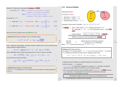
Abstract point of view:
Our notion of “problem”:
data space X, usually X ⊂ R n
result space Y , usually Y ⊂ R m
mapping (problem function) F : X ↦→ Y
x
X
data
Application to linear system of equations Ax = b, A ∈ K n,n , b ∈ K n :
“The problem:”
F
y
Y
results
data ˆ= system matrix A ∈ R n,n , right hand side vector b ∈ R n
➤ data space X = R n,n × R n with vector/matrix norms (→ Defs. 2.5.1,
2.5.2)
problem mapping (A,b) ↦→ F(A,b) := A −1 b , (for regular A)
Ôº½½ ¾º
(→ programme in C++ or FORTRAN)
Stability is a property of a particular algorithm for a problem
Numerical
Specific sequence of elementary operations
=
algorithm
Below: X, Y = normed vector spaces, e.g., X = R n , Y = R m
Definition 2.5.5 (Stable algorithm).
An algorithm ˜F for solving a problem F : X ↦→ Y is numerically stable, if for all x ∈ X its result
˜F(x) (affected by roundoff) is the exact result for “slightly perturbed” data:
∃C ≈ 1: ∀x ∈ X: ∃̂x ∈ X: ‖x − ̂x‖ ≤ Ceps ‖x‖ ∧ ˜F(x) = F(̂x) .
✬
✫
max
‖x‖ 2 =1 xH Ax = max
‖x‖ 2 =1 (Ux)H D(Ux) = max
‖y‖ 2 =1 yH Dy = max |d i| .
i=1,...,i
Corollary 2.5.4 (2-Matrixnorm and eigenvalues).
For A ∈ K m,n the 2-Matrixnorm ‖A‖ 2 is the square root of the largest (in modulus) eigenvalue
of A H A.
✷
✩
✪
Ôº½½ ¾º
• Judgement about the stability of an algorithm depends on the chosen norms !
• What is meant by C ≈ 1 in practice ?
C ≈ 1 ↔ C ≈ no. of elementary operations for computing ˜F(x): The longer a computation
takes the more accumulation of roundoff errors we are willing to tolerate.
• The use of computer arithmetic involves inevitable relative input errors (→ Ex. 2.4.5) of the size
ofeps. Moreover, in most applications the input data are also affected by other (e.g,
measurement) errors. Hence stability means that
Ôº½¾¼ ¾º
Roundoff errors affect the result in the same way as inevitable data errors.
➣ for stable algorithms roundoff errors are “harmless”.